ScreenR Example Analysis

Importing Package

knitr::opts_chunk$set(collapse = TRUE, comment = "#>")
library(ggplot2)
library(dplyr)

## 
## Attaching package: 'dplyr'

## The following objects are masked from 'package:stats':
## 
##     filter, lag

## The following objects are masked from 'package:base':
## 
##     intersect, setdiff, setequal, union

library(tidyr)

Introduction

The R package ScreenR has been developed to perform analysis of High-throughput RNA interference screening using pooled shRNA libraries and next generation sequencing.. Nowadays several short hairpin RNA (shRNA) libraries are commercial available, and in the last years the interest in this type of analysis, often called barcode screening, has greatly increased for their benefits both from a time-consuming point of view and for the possibility of carrying out screening on a large number of genes simultaneously. However, the bioinformatic analysis of this type of screening still lacks a golden standard. Here, ScreenR allows the user to carry out a preliminary quality check of the experiment, visually inspect the data and finally identify the most significant hits of the experiment through a series of plots and cross-statistical analyses.

Installation

Bioconductor

ScreenR requires several CRAN and Bioconductor R packages to be installed. Dependencies are usually handled automatically, when installing the package using the following commands:

if (!require("BiocManager", quietly = TRUE))
    install.packages("BiocManager")

BiocManager::install("ScreenR")

Github

The newest version can directly be installed from GitHub using the CRAN package devtools:

if (!require("devtools", quietly = TRUE))
   install.packages("devtools")

devtools::install_github("EmanuelSoda/ScreenR")

Analysis

Here is reported the ScreenR pipeline

Loading the package

After installation, loading the package is simple as :

library(ScreenR)
#> 
#> Welcome to ScreenR
#> --------------------------
#> 
#> See ?ScreenR for a list of
#> available functions.
#> 
#> Enjoy!
#>

Read Data

The input of ScreenR is a count table obtained from barcode alignment to the reference genome/library. A count table is usually the starting point of an RNA-seq deferentially expressed genes analysis and consists of a matrix containing reads count organized with:

Genes on the rows
Samples on the columns

For this vignette we will use as an example a Loss of Function Chemical lethality Genetic Screening performed using shRNA libraries where each gene is represented by ten slightly different shRNA each labeled with a unique barcode coming from an unpublished dataset generated using the Cellecta protocol.

First of all the data has to be read. Then another very important step is to set up the column names in the following way:

The first part of the string is the timepoint
The second is the type of sample (example: treated or control or the name of the treatment)
Third slot is a way to make each replicate unique (for example a letter or a number)

In the end we have

Time point_Type of sample_replicate

and for example we could have h24_control_1 which mean the first replicate of the control sample at 24 hour.

Since this dataset comes from a Chemical Synthetic Lethality experiments the samples treated with the drug combined with the shRNAs knockdown should present a decreased number of reads compared to the controls.

data(count_table)
data(annotation_table)

data <- count_table
colnames(data) <- c(
    "Barcode", "Time1", "Time2", "Time3_TRT_A", "Time3_TRT_B", "Time3_TRT_C",
    "Time3_CTRL_A", "Time3_CTRL_B", "Time3_CTRL_C", 
    "Time4_TRT_A", "Time4_TRT_B", "Time4_TRT_C", 
    "Time4_CTRL_A", "Time4_CTRL_B", "Time4_CTRL_C"
)
data <- data %>%
    dplyr::mutate(Barcode = as.factor(Barcode)) %>%
    dplyr::filter(Barcode != "*") %>%  
  tibble()


total_Annotation <- annotation_table

Object Creation

The second needed step is to create a ScreenR object from the count table. The ScreenR object is created using the function create_screenr_object() and will be used to store the most important information to perform the analysis. Most of the ScreenR function takes as main input the ScreenR object to perform the needed operation and return a result.

groups <- factor(c(
    "T1/T2", "T1/T2",
    "Time3_TRT", "Time3_TRT", "Time3_TRT",
    "Time3_CTRL", "Time3_CTRL", "Time3_CTRL",
    "Time4_TRT", "Time4_TRT", "Time4_TRT",
    "Time4_CTRL", "Time4_CTRL", "Time4_CTRL"
))


palette <- c("#66c2a5", "#fc8d62", rep("#8da0cb", 3), rep("#e78ac3", 3),
    rep("#a6d854", 3), rep("#ffd92f", 3))


object <- create_screenr_object(
    table = data, annotation = total_Annotation, groups = groups,
    replicates = ""
)

Removing all zero rows

object <- remove_all_zero_row(object)

Computing the needed tables

Once the object is created, the data must be normalized to start the analysis. ScreenR uses Counts Per Million (CPM) normalization which has the following mathematical expression:

\[CPM = \frac{Number \; of \; mapped \; reads \; to \; a \; barcode} { \sum_{sample}{Number\; of \;mapped \; reads}} *10^{6}\]

The number of reads mapped for each barcode in a sample are normalized by the number of reads in that sample and multiplied by one million.

This information is store in a data table which is a tidy version of the original count table and will be used throughout the analysis.

object <- normalize_data(object)
object <- compute_data_table(object)

Quality Check

The first step to perform when dealing with sequencing data is to check the quality of the samples. In ScreenR this can be done using several methods.

Mapped Reads

The total number of mapped reads can be displayed with a barplot with the formula.

plot <- plot_mapped_reads(object, palette) +
    ggplot2::coord_flip() +
    ggplot2::scale_y_continuous(labels = scales::comma) +
    ggplot2::theme(legend.position = "none") +
    ggplot2::ggtitle("Number of Mapped Reads in each sample")

plot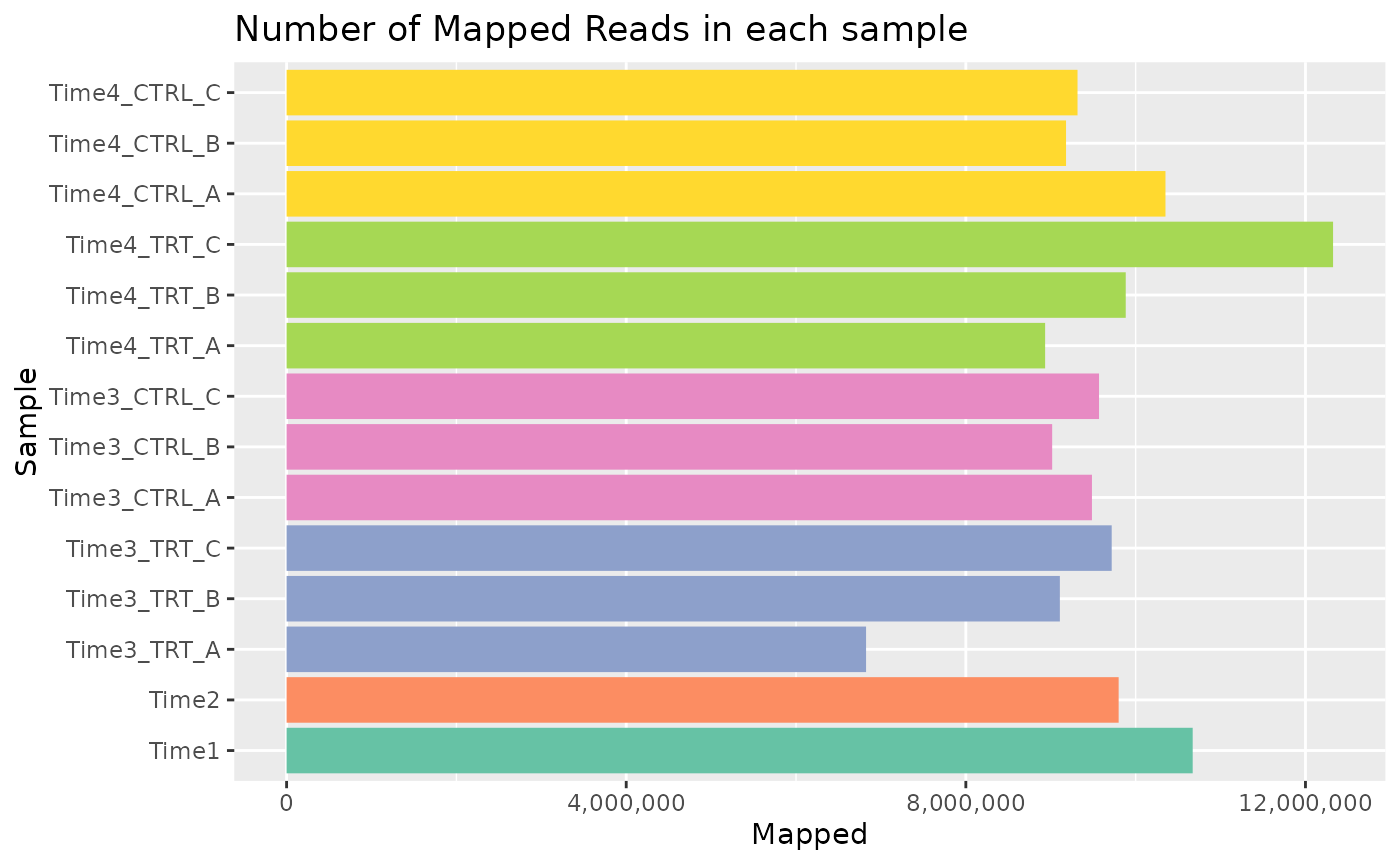

For example the distribution can be seen using both boxplots or density plots.

#### Boxplot Mapped Reads

plot <- plot_mapped_reads_distribution(
    object, palette,
    alpha = 0.8,
    type = "boxplot"
) +
    coord_flip() +
    theme(legend.position = "none") 

plot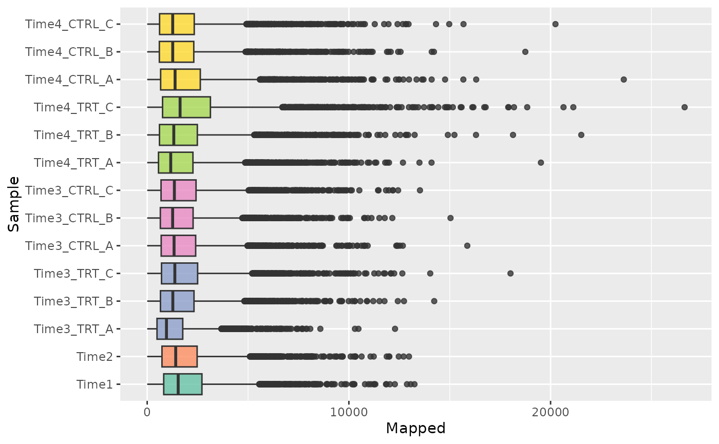

Density plot

plot <- plot_mapped_reads_distribution(
    object, palette,
    alpha = 0.5,
    type = "density"
) +
    ggplot2::theme(legend.position = "none") 

plot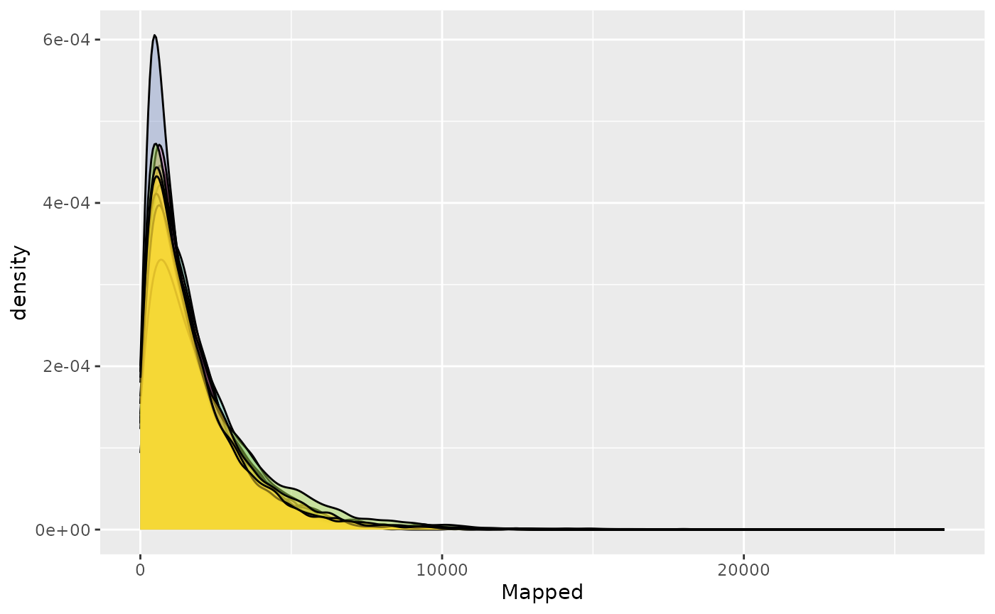

Barcode Lost

Another very important quality check when a Genetic Screening is performed is to check the barcode lost during the experiment, meaning the barcode that after different time points or treatments results in reads count equal to zero. ScreenR implements a function able to compute and plot the number of barcodes lost for each samples.

plot <- plot_barcode_lost(screenR_Object = object, palette = palette) +
    ggplot2::coord_flip()
plot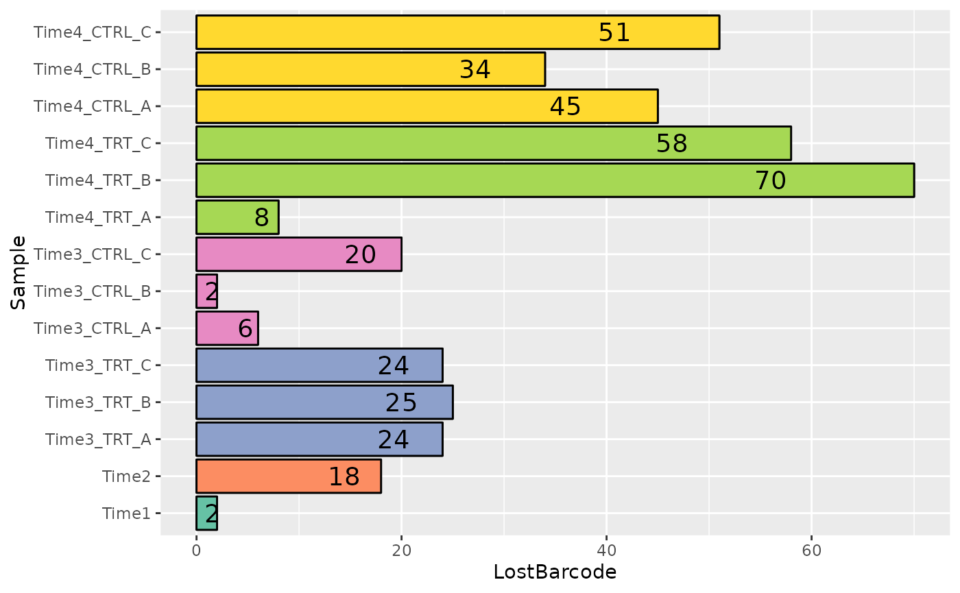

Moreover it is important to check if the lost barcodes in a sample all belong to the same gene, in order to verify that an adequate number of barcodes per gene are still present. This can be done by visualizing the number of barcode lost in a sample by gene.

plot <- plot_barcode_lost_for_gene(object,
    samples = c("Time4_TRT_C", "Time4_CTRL_C")
)
plot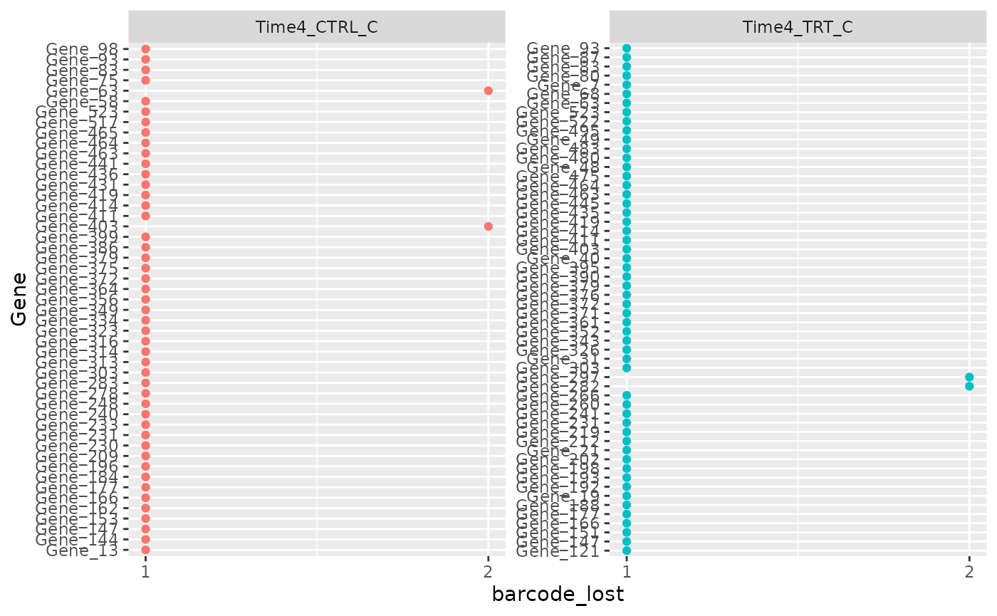

Plot MDS

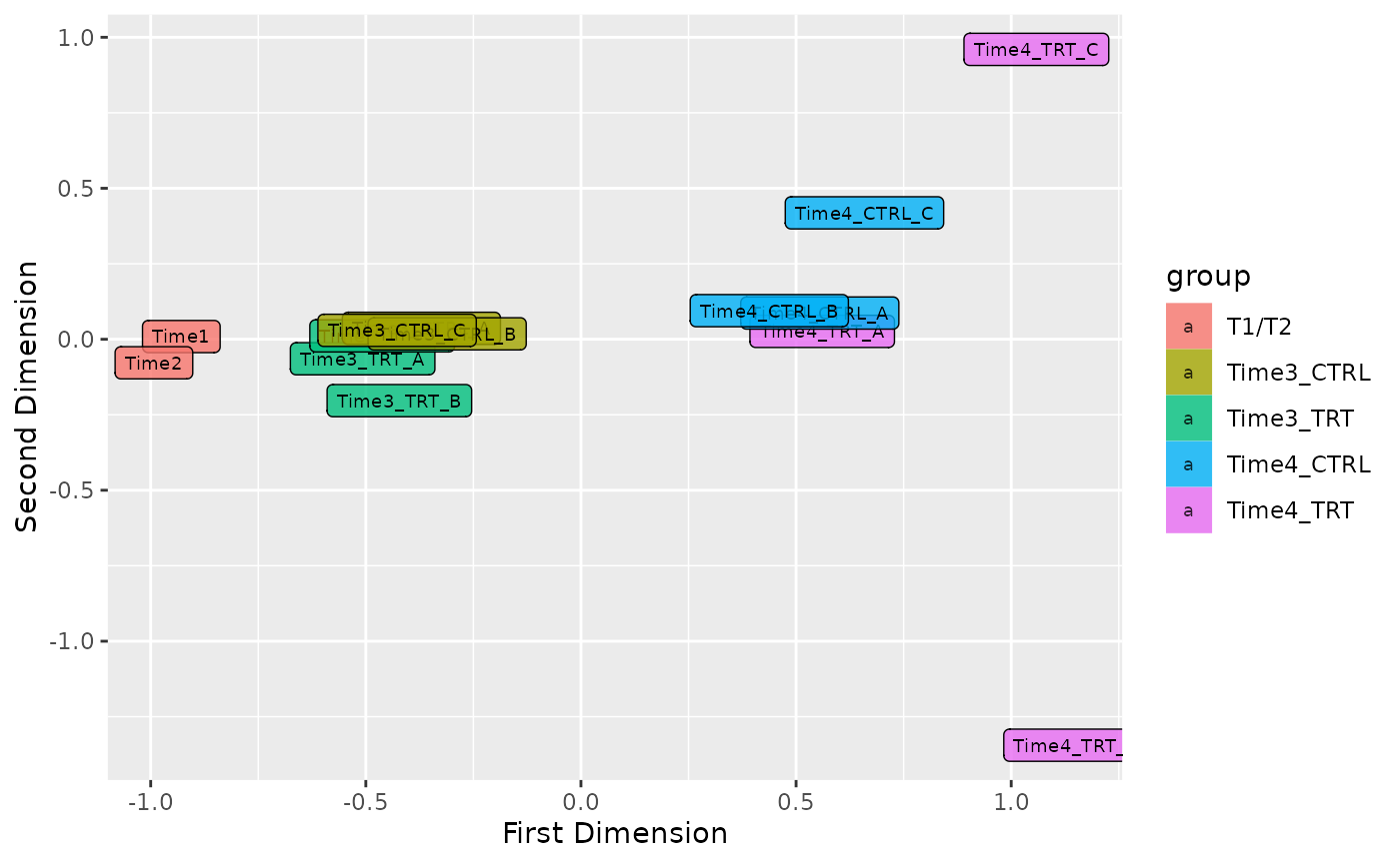
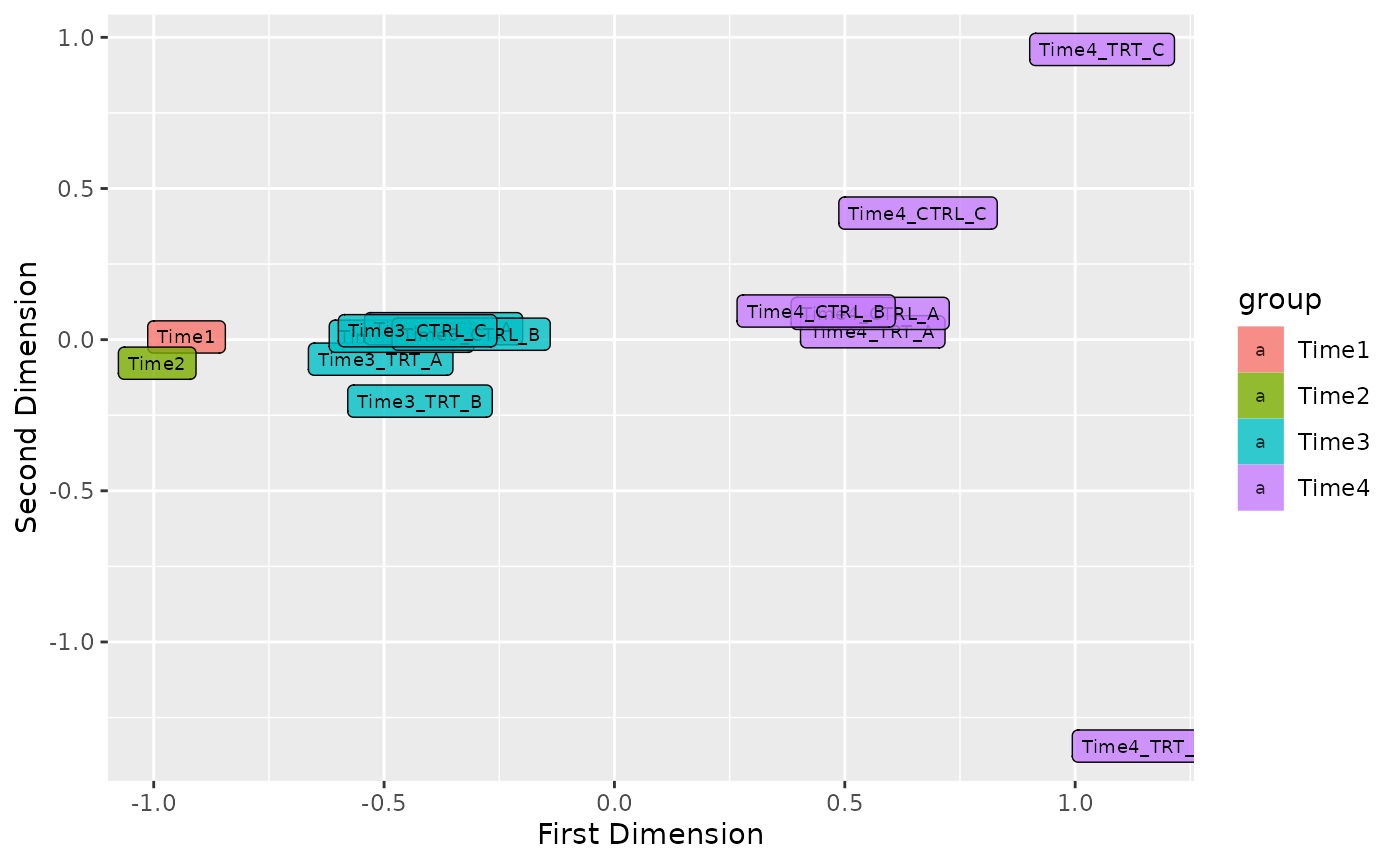
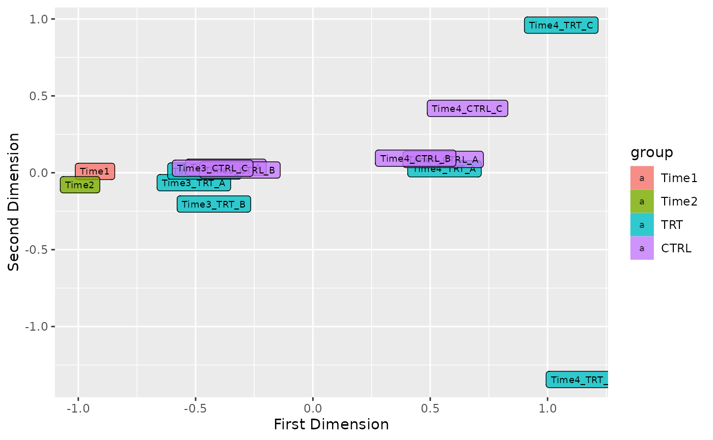
In order to see the samples clusterization an initial MDS analysis can be conducted. In ScreenR this can be done using the plot_mds function and the user can decide the color code of the graph in order to highlight the trend of the samples based on replicates, treatment or timepoints simply by modifying the field levels in the plot_mds function.

For Sample

plot_mds(screenR_Object = object)

For Treatment

group_table <- get_data_table(object)   %>%
    select(Sample, Day, Treatment) %>%
    distinct()
#> ScreenR normalized data table containing:
#>  74438 rows
#>  9 columns

group_treatment <- group_table$Treatment

plot_mds(
    screenR_Object = object,
    groups = factor(x = group_treatment, levels = unique(group_treatment))
)

For Day

group_day <- group_table$Day

plot_mds(
    screenR_Object = object,
    groups = factor(x = group_day, levels = unique(group_day))
)

Statistical Analysis

Once the various steps of the quality check have been passed, the actual statistical analysis can begin. The statistical Analysis of ScreenR is based on three different methods:

Z-score hit

In order to compute the Z-score, first a list of metrics has to be computed. In particular a Log2FC is computed for the treated vs control samples in the different conditions. This can be done using the function compute_metrics(). Here is reported an example of treated vs control in different day.

Then the different distribution of the Z-score can be plotted using the plot_zscore_distribution function.

# 2DG
data_with_measure_TRT <- list(
    Time3 = compute_metrics(
        object,
        control = "CTRL", treatment = "TRT",
        day = "Time3"
    ),
    Time4 = compute_metrics(
        object,
        control = "CTRL", treatment = "TRT",
        day = "Time4"
    )
)

plot_zscore_distribution(data_with_measure_TRT, alpha = 0.8)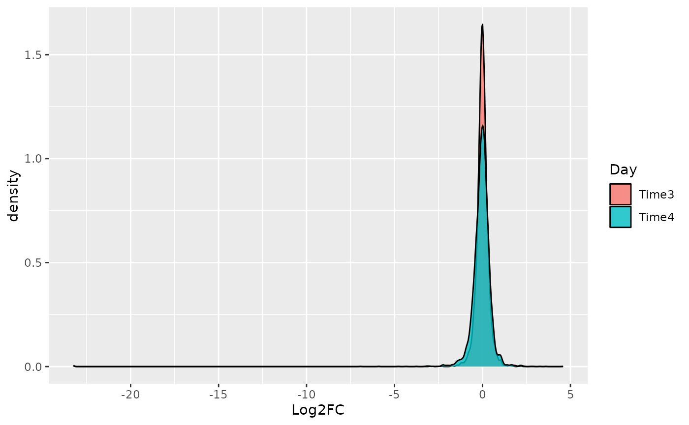

Z-score hit

Based on these metrics the Z-score hit identification can be computed using the find_zscore_hit function.

zscore_hit_TRT <- list(
    Time3 = find_zscore_hit(
        table_treate_vs_control = data_with_measure_TRT$Time3,
        number_barcode = 6, metric = "median"
    ),
    Time4 = find_zscore_hit(
        table_treate_vs_control = data_with_measure_TRT$Time4,
        number_barcode = 6, metric = "median"
    )
)
zscore_hit_TRT
#> $Time3
#> # A tibble: 83 × 2
#>    Gene     numberOfBarcode
#>    <chr>              <int>
#>  1 Gene_1                 7
#>  2 Gene_11                7
#>  3 Gene_116               8
#>  4 Gene_120               8
#>  5 Gene_121               7
#>  6 Gene_128               8
#>  7 Gene_15                7
#>  8 Gene_156               8
#>  9 Gene_158               7
#> 10 Gene_160               7
#> # ℹ 73 more rows
#> 
#> $Time4
#> # A tibble: 97 × 2
#>    Gene     numberOfBarcode
#>    <chr>              <int>
#>  1 Gene_107               7
#>  2 Gene_121               8
#>  3 Gene_125               7
#>  4 Gene_126               7
#>  5 Gene_134               7
#>  6 Gene_138               7
#>  7 Gene_139               7
#>  8 Gene_14                7
#>  9 Gene_147               8
#> 10 Gene_148               9
#> # ℹ 87 more rows

CAMERA

The same can be done with the CAMERA hit using the function find_camera_hit.

matrix_model <- model.matrix(~ groups)
colnames(matrix_model) <- unique(groups)


camera_hit_TRT <- list(
    Time3 = find_camera_hit(
        screenR_Object = object, matrix_model = matrix_model,
        contrast = "Time3_TRT",
    ),
    Time4 = find_camera_hit(
        screenR_Object = object, matrix_model = matrix_model,
        contrast = "Time4_TRT"
    )
)

camera_hit_TRT
#> $Time3
#> # A tibble: 258 × 5
#>    Gene     NGenes Direction   PValue      FDR
#>    <chr>     <dbl> <fct>        <dbl>    <dbl>
#>  1 Gene_372     12 Down      3.80e-15 1.93e-12
#>  2 Gene_364     12 Down      7.23e-15 1.93e-12
#>  3 Gene_374     10 Down      3.55e- 7 6.32e- 5
#>  4 Gene_282     10 Down      2.24e- 4 2.40e- 2
#>  5 Gene_75      10 Down      7.59e- 4 6.76e- 2
#>  6 Gene_323     10 Down      1.45e- 3 1.11e- 1
#>  7 Gene_179     10 Down      1.68e- 3 1.12e- 1
#>  8 Gene_117     10 Down      1.10e- 2 4.23e- 1
#>  9 Gene_228     10 Down      1.49e- 2 4.97e- 1
#> 10 Gene_211     10 Down      1.84e- 2 5.77e- 1
#> # ℹ 248 more rows
#> 
#> $Time4
#> # A tibble: 241 × 5
#>    Gene     NGenes Direction   PValue      FDR
#>    <chr>     <dbl> <fct>        <dbl>    <dbl>
#>  1 Gene_364     12 Down      1.13e-24 6.03e-22
#>  2 Gene_372     12 Down      3.46e-21 9.24e-19
#>  3 Gene_374     10 Down      9.55e- 8 1.70e- 5
#>  4 Gene_323     10 Down      7.27e- 7 9.70e- 5
#>  5 Gene_282     10 Down      6.22e- 6 6.64e- 4
#>  6 Gene_75      10 Down      1.76e- 5 1.57e- 3
#>  7 Gene_296     10 Down      1.31e- 4 1.00e- 2
#>  8 Gene_80      10 Down      5.72e- 4 3.82e- 2
#>  9 Gene_54      10 Down      7.94e- 3 3.26e- 1
#> 10 Gene_179     10 Down      1.13e- 2 3.94e- 1
#> # ℹ 231 more rows

ROAST

Last but not least this is done also for the ROAST hit using the function
find_roast_hit.

roast_hit_TRT <- list(
    Time3 = find_roast_hit(
        screenR_Object = object, matrix_model = matrix_model,
        contrast = "Time3_TRT", 
    ),
    Time4 = find_roast_hit(
        screenR_Object = object, matrix_model = matrix_model,
        contrast = "Time4_TRT"
    )
)

roast_hit_TRT
#> $Time3
#> # A tibble: 30 × 9
#>    Gene   NGenes PropDown PropUp Direction PValue     FDR PValue.Mixed FDR.Mixed
#>    <chr>   <int>    <dbl>  <dbl> <fct>      <dbl>   <dbl>        <dbl>     <dbl>
#>  1 Gene_…     12    0.917    0   Down      0.0001 0.00668       0.0001    0.0134
#>  2 Gene_…     12    0.833    0   Down      0.0001 0.00668       0.0001    0.0134
#>  3 Gene_…     10    0.7      0   Down      0.0001 0.00668       0.0004    0.0623
#>  4 Gene_…     10    0.5      0.1 Down      0.0003 0.0267        0.0018    0.104 
#>  5 Gene_…     10    0.3      0   Down      0.0005 0.0386        0.0182    0.235 
#>  6 Gene_…     10    0.4      0   Down      0.0007 0.0386        0.0223    0.242 
#>  7 Gene_…     10    0.5      0   Down      0.001  0.0507        0.0252    0.263 
#>  8 Gene_…     10    0.2      0   Down      0.0047 0.166         0.0705    0.399 
#>  9 Gene_…     10    0.3      0.1 Down      0.0076 0.231         0.0098    0.156 
#> 10 Gene_…     10    0.2      0   Down      0.0086 0.231         0.0214    0.242 
#> # ℹ 20 more rows
#> 
#> $Time4
#> # A tibble: 106 × 9
#>    Gene   NGenes PropDown PropUp Direction PValue     FDR PValue.Mixed FDR.Mixed
#>    <chr>   <int>    <dbl>  <dbl> <fct>      <dbl>   <dbl>        <dbl>     <dbl>
#>  1 Gene_…     12      1      0   Down      0.0001 0.00191       0.0001  0.000861
#>  2 Gene_…     12      1      0   Down      0.0001 0.00191       0.0001  0.000861
#>  3 Gene_…     10      0.9    0   Down      0.0001 0.00191       0.0001  0.000861
#>  4 Gene_…     10      0.7    0   Down      0.0001 0.00191       0.0001  0.000861
#>  5 Gene_…     10      0.7    0   Down      0.0001 0.00191       0.0001  0.000861
#>  6 Gene_…     10      0.7    0   Down      0.0001 0.00191       0.0001  0.000861
#>  7 Gene_…     10      0.6    0.1 Down      0.0001 0.00191       0.0008  0.00413 
#>  8 Gene_…     10      0.6    0   Down      0.0001 0.00191       0.0011  0.00496 
#>  9 Gene_…     10      0.5    0.2 Down      0.0001 0.00191       0.0003  0.00212 
#> 10 Gene_…     10      0.4    0   Down      0.0001 0.00191       0.0002  0.00163 
#> # ℹ 96 more rows

Find Common Hit

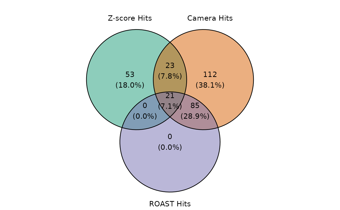
ScreenR considers as final hit only the one result as candidate hit in all three statistical methods. However this is a particularly stringent method and in some cases leads to a small number of results. For this reason the user can also decide to opt for a less stringent method that considers only the hits present in at least two of the statistical methods. The two different strategies can be computed with the function::

common_hit_TRT_at_least_2: considering candidate Hits the one present in at least two of the three methods (less stringent)
common_hit_TRT_at_least_3: considering candidate Hits the one present in all of the three methods

common_hit_TRT_at_least_2 <- list(
    Time3 = find_common_hit(
        zscore_hit_TRT$Time3, camera_hit_TRT$Time3, roast_hit_TRT$Day3,
        common_in = 2
    ),
    Time4 = find_common_hit(
        zscore_hit_TRT$Time4, camera_hit_TRT$Time4, roast_hit_TRT$Day6,
        common_in = 2
    )
)

common_hit_TRT_at_least_3 <- list(
    Time3 = find_common_hit(
        zscore_hit_TRT$Time3, camera_hit_TRT$Time3, roast_hit_TRT$Time3,
        common_in = 3
    ),
    Time4 = find_common_hit(
        zscore_hit_TRT$Time4, camera_hit_TRT$Time4, roast_hit_TRT$Time4,
        common_in = 3
    )
)

Plot common hit

The intersection of the hits found by the three statistical methods can be easily visualized using the plot_common_hit function.

plot_common_hit(
    hit_zscore = zscore_hit_TRT$Time4, hit_camera = camera_hit_TRT$Time4,
    roast_hit_TRT$Time4, show_elements = FALSE, show_percentage = TRUE
)

As we all know, when we deal with statistical methods the is the possibility of type I error also known as “false positive”. For this reason is important to visualize the results obtained. This can be done by visualizing the trend of the candidate hits obtained using the function plot_trend.

candidate_hits <- common_hit_TRT_at_least_2$Time3

plot_trend(screenR_Object = object, 
           genes = candidate_hits[1], 
           nrow = 2, ncol = 2, 
           group_var = c("Time1", "Time2", "TRT"))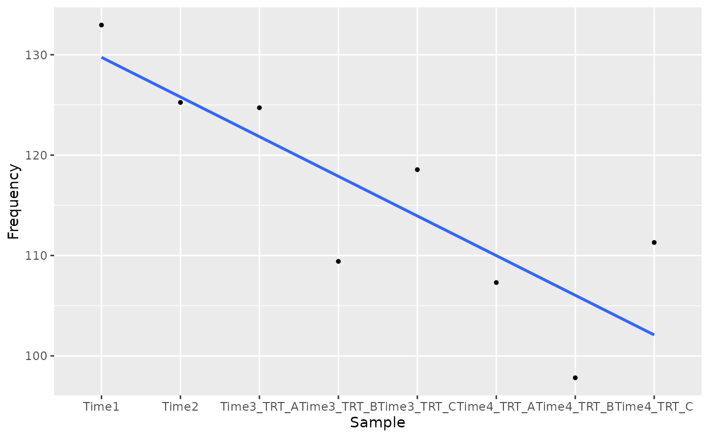


plot_trend(screenR_Object = object, 
           genes = candidate_hits[2], 
           nrow = 2, ncol = 2, 
           group_var = c("Time1", "Time2", "TRT"))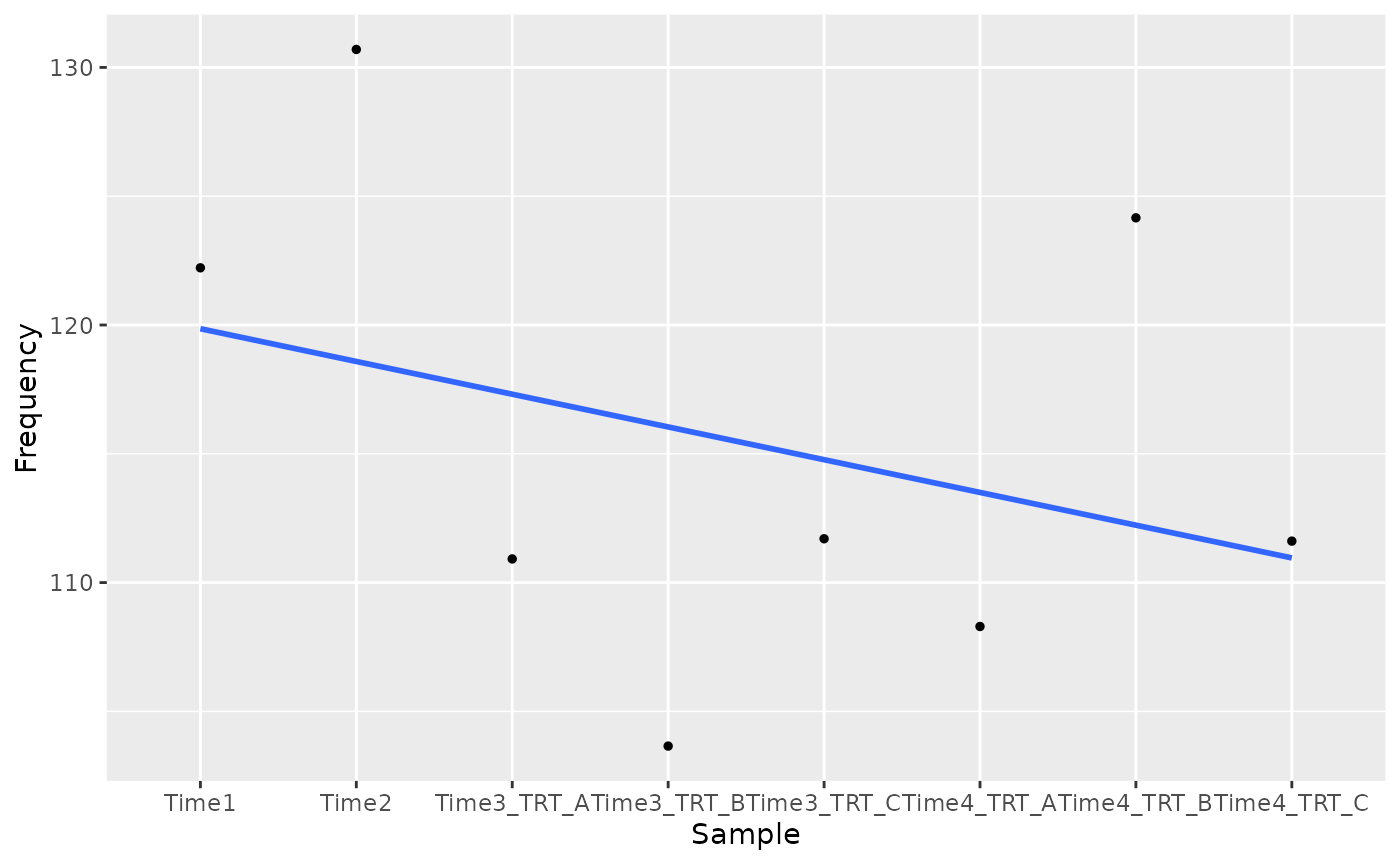

sessionInfo()
#> R version 4.3.1 (2023-06-16)
#> Platform: x86_64-pc-linux-gnu (64-bit)
#> Running under: Ubuntu 22.04.3 LTS
#> 
#> Matrix products: default
#> BLAS:   /usr/lib/x86_64-linux-gnu/openblas-pthread/libblas.so.3 
#> LAPACK: /usr/lib/x86_64-linux-gnu/openblas-pthread/libopenblasp-r0.3.20.so;  LAPACK version 3.10.0
#> 
#> locale:
#>  [1] LC_CTYPE=C.UTF-8       LC_NUMERIC=C           LC_TIME=C.UTF-8       
#>  [4] LC_COLLATE=C.UTF-8     LC_MONETARY=C.UTF-8    LC_MESSAGES=C.UTF-8   
#>  [7] LC_PAPER=C.UTF-8       LC_NAME=C              LC_ADDRESS=C          
#> [10] LC_TELEPHONE=C         LC_MEASUREMENT=C.UTF-8 LC_IDENTIFICATION=C   
#> 
#> time zone: UTC
#> tzcode source: system (glibc)
#> 
#> attached base packages:
#> [1] stats     graphics  grDevices utils     datasets  methods   base     
#> 
#> other attached packages:
#> [1] ScreenR_0.99.55  tidyr_1.3.0      dplyr_1.1.3      ggplot2_3.4.3   
#> [5] BiocStyle_2.28.1
#> 
#> loaded via a namespace (and not attached):
#>  [1] sass_0.4.7          utf8_1.2.3          generics_0.1.3     
#>  [4] stringi_1.7.12      lattice_0.21-8      digest_0.6.33      
#>  [7] magrittr_2.0.3      evaluate_0.21       grid_4.3.1         
#> [10] bookdown_0.35       fastmap_1.1.1       Matrix_1.5-4.1     
#> [13] rprojroot_2.0.3     jsonlite_1.8.7      limma_3.56.2       
#> [16] BiocManager_1.30.22 mgcv_1.8-42         purrr_1.0.2        
#> [19] fansi_1.0.4         scales_1.2.1        textshaping_0.3.6  
#> [22] jquerylib_0.1.4     cli_3.6.1           rlang_1.1.1        
#> [25] splines_4.3.1       munsell_0.5.0       withr_2.5.0        
#> [28] cachem_1.0.8        yaml_2.3.7          tools_4.3.1        
#> [31] memoise_2.0.1       colorspace_2.1-0    locfit_1.5-9.8     
#> [34] ggvenn_0.1.10       vctrs_0.6.3         R6_2.5.1           
#> [37] lifecycle_1.0.3     stringr_1.5.0       edgeR_3.42.4       
#> [40] fs_1.6.3            ragg_1.2.5          pkgconfig_2.0.3    
#> [43] desc_1.4.2          pkgdown_2.0.7       pillar_1.9.0       
#> [46] bslib_0.5.1         gtable_0.3.4        glue_1.6.2         
#> [49] Rcpp_1.0.11         systemfonts_1.0.4   xfun_0.40          
#> [52] tibble_3.2.1        tidyselect_1.2.0    knitr_1.44         
#> [55] farver_2.1.1        nlme_3.1-162        patchwork_1.1.3    
#> [58] htmltools_0.5.6     labeling_0.4.3      rmarkdown_2.25     
#> [61] compiler_4.3.1

Emanuel Michele Soda

Elena Ceccacci

2023-09-22

Importing Package

Introduction

Installation

Bioconductor

Github

Analysis

Loading the package

Read Data

Object Creation

Removing all zero rows

Computing the needed tables

Quality Check

Mapped Reads

Density plot

Barcode Lost

Plot MDS

For Sample

For Treatment

For Day

Statistical Analysis

Z-score hit

Z-score hit

CAMERA

ROAST

Find Common Hit

Plot common hit