Tutorial 4: CRISPR-Cas9 screens

About this tutorial

ScreenR was written for shRNA screens, but CRISPR-Cas9 knockout screens produce the same kind of data: a table of read counts, one row for each guide RNA (sgRNA) and one column for each sample. In ScreenR an sgRNA is simply a “barcode”, and everything in the other tutorials applies. This tutorial goes through a CRISPR dropout screen step by step and shows what is specific to CRISPR:

installing ScreenR and, optionally, CRISPRcleanR;
describing a time-course dropout screen (T0 and later time points);
choosing the thresholds on the number of sgRNAs per gene;
checking the quality of the screen with essential and non-essential reference genes;
measuring the efficiency of the sgRNAs;
correcting the copy-number bias of CRISPR-Cas9 with CRISPRcleanR;
finding the hits, using the non-essential genes as reference, and checking the sgRNAs of each hit;
positive-selection screens.

	shRNA screen	CRISPR-Cas9 knockout screen
Reagent (a “barcode” in ScreenR)	shRNA	sgRNA
Reagents per gene	often 5 to 25	usually 3 to 6 (4 in TKOv3 and Brunello)
Typical design	treated vs control at each time point	late time point vs T0 or plasmid
Gene-independent effects	seed (off-target) effects	DNA cutting: copy-number and proximity bias
Good null reference	non-essential genes	non-essential genes (non-targeting sgRNAs do not cut, so they are not a good null)

Installation

ScreenR is on Bioconductor:

if (!requireNamespace("BiocManager", quietly = TRUE)) {
    install.packages("BiocManager")
}
BiocManager::install("ScreenR")

The copy-number correction uses the CRISPRcleanR package (Iorio et al. 2018). It is optional: everything else in this tutorial works without it. CRISPRcleanR is not on CRAN or Bioconductor, so it is installed from GitHub; BiocManager::install() also installs its Bioconductor dependencies:

BiocManager::install("francescojm/CRISPRcleanR")

crisprcleanr_available() tells whether it is installed:

library(ScreenR)
library(dplyr)
library(ggplot2)

crisprcleanr_available()

The plots of ScreenR have no theme of their own; one is chosen for the whole tutorial with theme_set():

theme_set(theme_light(base_size = 12))

CRISPRcleanR is not installed where this tutorial was built: the code of the copy-number correction is shown but not run, and its results are read from a precomputed table.

The data

hap1_count_table comes from a genome-wide CRISPR-Cas9 knockout screen of HAP1 cells with the TKOv3 library (Hart et al. 2017): the T0 sample and three replicates after 3 and 18 days of growth. Cells that lose a gene needed for growth (an essential gene) are lost over time, so the sgRNAs of essential genes are depleted at day 18. To keep the package small the dataset is a subset of the 70,877 sgRNAs of the library (see ?hap1_count_table).

data(hap1_count_table)
data(hap1_annotation_table)
head(hap1_count_table)
#>                     Barcode  T0 T3_A T3_B T3_C T18_A T18_B T18_C
#> 1 EGFP_TGGTTGTCGGGCAGCAGCAC 537  222  150  216   243   115   304
#> 2 EGFP_GGTTGTCGGGCAGCAGCACG 210  197   92  125   195   177   115
#> 3 EGFP_TTCAAGTCCGCCATGCCCGA 517  423  255  282   329   309   433
#> 4 EGFP_CGGCGGTCACGAACTCCAGC 278  167   54  120   165   184    65
#> 5 EGFP_GGTGCCCATCCTGGTCGAGC  83   99   41   19   107   103    44
#> 6 EGFP_GAAGTTCGAGGGCGACACCC 268  145  153  204   133   295   228
head(hap1_annotation_table)
#>                     Barcode Gene Chromosome Strand Start End   Class
#> 1 EGFP_TGGTTGTCGGGCAGCAGCAC EGFP       <NA>   <NA>    NA  NA control
#> 2 EGFP_GGTTGTCGGGCAGCAGCACG EGFP       <NA>   <NA>    NA  NA control
#> 3 EGFP_TTCAAGTCCGCCATGCCCGA EGFP       <NA>   <NA>    NA  NA control
#> 4 EGFP_CGGCGGTCACGAACTCCAGC EGFP       <NA>   <NA>    NA  NA control
#> 5 EGFP_GGTGCCCATCCTGGTCGAGC EGFP       <NA>   <NA>    NA  NA control
#> 6 EGFP_GAAGTTCGAGGGCGACACCC EGFP       <NA>   <NA>    NA  NA control

The annotation has the gene of each sgRNA and its position in the genome (used by CRISPRcleanR), and a Class column that tells the core essential and non-essential reference genes, the controls and the other genes.

Creating the ScreenR object

The sample names (T0, T3_A, …) do not follow the Day_Treatment_Replicate convention of ScreenR, so the samples are described with a sample_table. T0, T3 and T18 are the time points (the Day column). A dropout screen has no treatment: the cells only grow, and the comparison is between time points, so every sample has the same Treatment, here "Untreated". The groups (used by the statistical models) are the time points. The palettes give each time point (and each sample) the same color in every plot.

samples <- data.frame(
    Sample = colnames(hap1_count_table)[-1],
    Day = c("T0", "T3", "T3", "T3", "T18", "T18", "T18"),
    Treatment = "Untreated"
)
samples
#>   Sample Day Treatment
#> 1     T0  T0 Untreated
#> 2   T3_A  T3 Untreated
#> 3   T3_B  T3 Untreated
#> 4   T3_C  T3 Untreated
#> 5  T18_A T18 Untreated
#> 6  T18_B T18 Untreated
#> 7  T18_C T18 Untreated
time_colors <- c(T0 = "#999999", T3 = "#7570B3", T18 = "#D95F02")
object <- create_screenr_object(
    table = hap1_count_table,
    annotation = hap1_annotation_table,
    groups = factor(samples$Day, levels = c("T0", "T3", "T18")),
    sample_table = samples,
    palettes = list(
        Day = time_colors, Group = time_colors,
        Sample = c(T0 = "#999999", T3_A = "#9E9AC8", T3_B = "#7570B3",
            T3_C = "#54278F", T18_A = "#FDAE6B", T18_B = "#D95F02",
            T18_C = "#A63603")
    )
)
object <- remove_all_zero_row(object)
object
#> class: screenr_object 
#> dim: 13598 7 
#> metadata(2): screenr_layout palettes
#> assays(1): counts
#> rownames(13598): EGFP_TGGTTGTCGGGCAGCAGCAC EGFP_GGTTGTCGGGCAGCAGCACG
#>   ... luciferase_GGCTATGAAGAGATACGCCC luciferase_GGCATGCGAGAATCTGACGC
#> rowData names(7): Barcode Gene ... End Class
#> colnames(7): T0 T3_A ... T18_B T18_C
#> colData names(4): Sample Day Treatment Group
#> normalization: none (run normalize_data())

How many sgRNAs per gene?

Several functions test a gene only if it has enough barcodes: number_barcode in find_camera_hit(), find_roast_hit(), find_time_hit() and plot_barcode_hit() (genes need more than number_barcode barcodes, default 3) and min_barcodes in find_gene_zscore_hit() (genes need at least min_barcodes, default 3). These defaults were chosen for shRNA libraries. barcodes_per_gene() shows what the library has:

per_gene <- barcodes_per_gene(object)
table(per_gene$NBarcodes)
#> 
#>    1    2    3    4   22   24   94 
#>   52   51   88 3260    1    1    1

Most genes have 4 sgRNAs. With number_barcode = 3, genes that lost one sgRNA (and genes designed with 3) are not tested; when this excludes many genes the functions give a warning that suggests a better value, so it is safe to start from the defaults. Here number_barcode = 2 (at least 3 sgRNAs) keeps almost every gene.

Quality control

The general quality control of Tutorial 2 applies to CRISPR screens, with any sample names and time points.

Sequencing depth

plot_mapped_reads() shows the number of reads of each sample. Samples with far fewer reads than the others are less reliable:

plot_mapped_reads(object)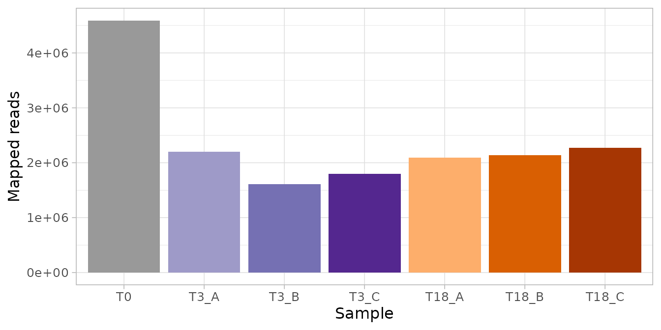

The T0 sample was sequenced about twice as deeply as the others, which is common: it is the reference of every comparison. Every sample has at least 1.6 million reads, more than 100 for each sgRNA of this subset.

plot_mapped_reads_distribution() shows the distribution of the reads of the sgRNAs in each sample:

plot_mapped_reads_distribution(object)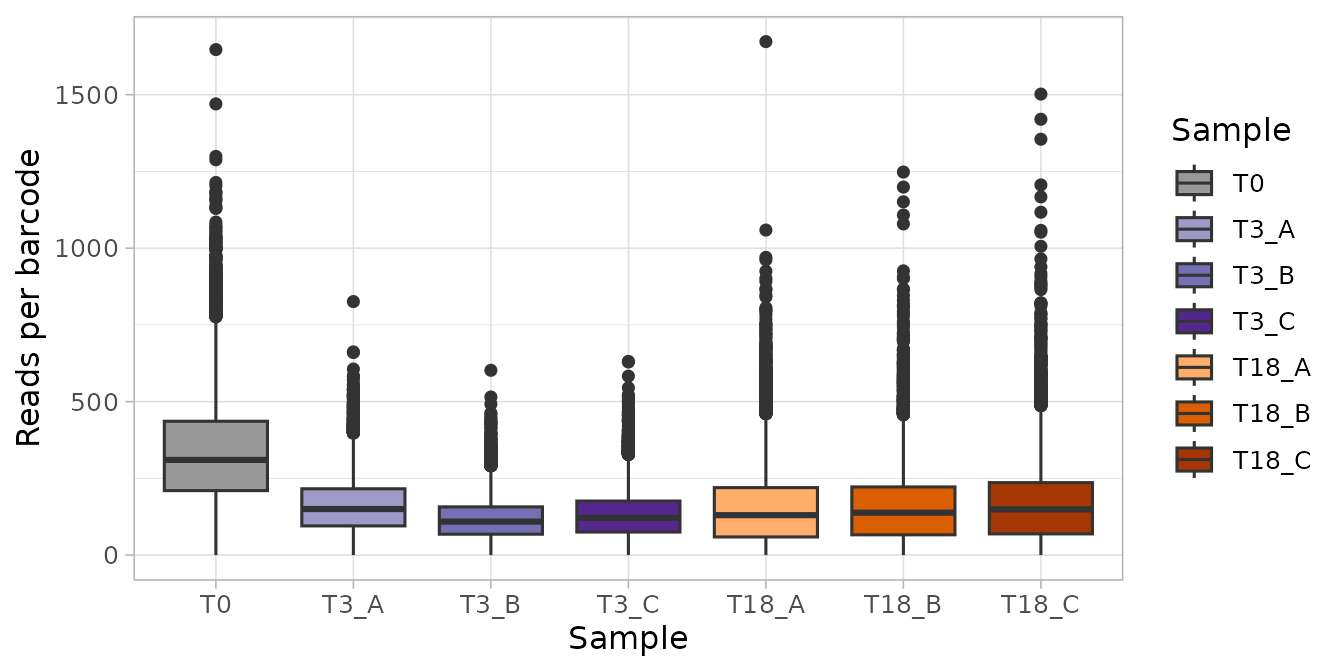

plot_mapped_reads_distribution(object, type = "density", alpha = 0.3)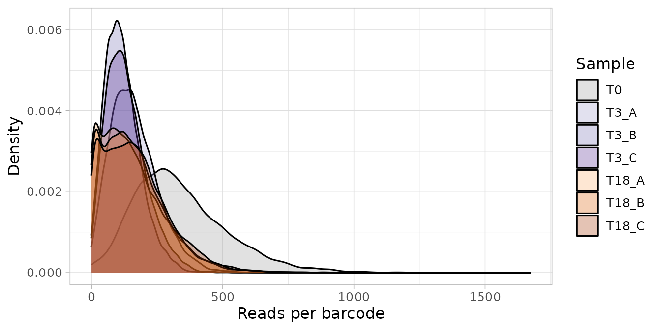

The counts are raw, so the T0 sample, sequenced more deeply, is shifted to the right. At day 18 the distribution is wider than at day 3, with more sgRNAs close to 0: the sgRNAs of the essential genes are dropping out.

Lost sgRNAs

barcode_lost() counts the sgRNAs with no reads in each sample and plot_barcode_lost() shows them. At T0 almost every sgRNA should be present: an sgRNA missing there was not represented in the library and cannot be measured.

barcode_lost(object)
#> # A tibble: 7 × 2
#>   Sample LostBarcode
#>   <fct>        <int>
#> 1 T0              26
#> 2 T3_A            47
#> 3 T3_B            48
#> 4 T3_C            63
#> 5 T18_A          456
#> 6 T18_B          301
#> 7 T18_C          296
plot_barcode_lost(object) +
    scale_x_discrete(guide = guide_axis(angle = 45))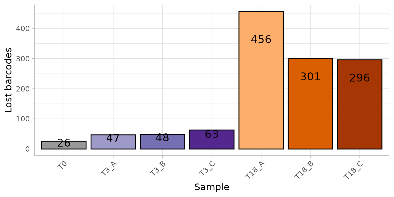

In a shRNA screen many lost barcodes are a warning; in a CRISPR dropout screen the sgRNAs lost at the late time point are expected, because the cells that carry the sgRNAs of essential genes are gone. count_mapped_reads() gives the reads of each sgRNA in each sample, so the lost sgRNAs can be assigned to the reference genes (defined in the quality section below):

data(hart_reference_genes)
essential <- hart_reference_genes$Gene[
    hart_reference_genes$Class == "core essential"]
nonessential <- hart_reference_genes$Gene[
    hart_reference_genes$Class == "non-essential"]
count_mapped_reads(object) %>%
    filter(Mapped == 0) %>%
    mutate(
        Gene = hap1_annotation_table$Gene[
            match(Barcode, hap1_annotation_table$Barcode)],
        Class = case_when(
            Gene %in% essential ~ "Core essential",
            Gene %in% nonessential ~ "Non-essential",
            TRUE ~ "Other"
        )
    ) %>%
    dplyr::count(Sample, Class) %>%
    tidyr::pivot_wider(names_from = Class, values_from = n, values_fill = 0)
#> # A tibble: 7 × 4
#>   Sample `Core essential` `Non-essential` Other
#>   <fct>             <int>           <int> <int>
#> 1 T0                    7               5    14
#> 2 T3_A                 16              11    20
#> 3 T3_B                 16              12    20
#> 4 T3_C                 26              12    25
#> 5 T18_A               362              17    77
#> 6 T18_B               238              12    51
#> 7 T18_C               240              11    45

At day 18 most lost sgRNAs target core essential genes, and very few target non-essential genes: the losses are the effect of the screen, not a technical problem. plot_barcode_lost_for_gene() (see Tutorial 2) lists the genes that lost sgRNAs in chosen samples; at day 18 they are hundreds, so it is more useful at T0, to find the genes that were poorly represented from the start:

plot_barcode_lost_for_gene(object, samples = "T0")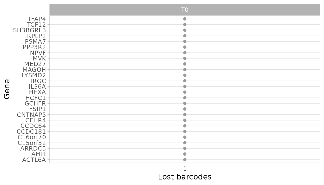

Each of these genes lost a single sgRNA at T0 and is still measured with the others.

Library representation and replicates

The library should be evenly represented at T0 (low Gini index) and the replicates should agree:

plot_gini(object)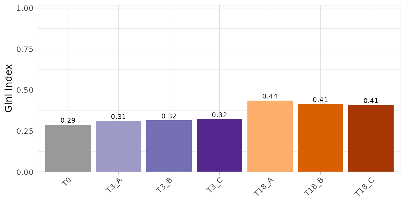

The plots so far use the raw counts. The correlation between replicates and the sample plots below compare normalized counts, so the counts are normalized first (counts per million; the choice of the normalization is discussed below):

object <- normalize_data(object)

plot_replicate_correlation(object)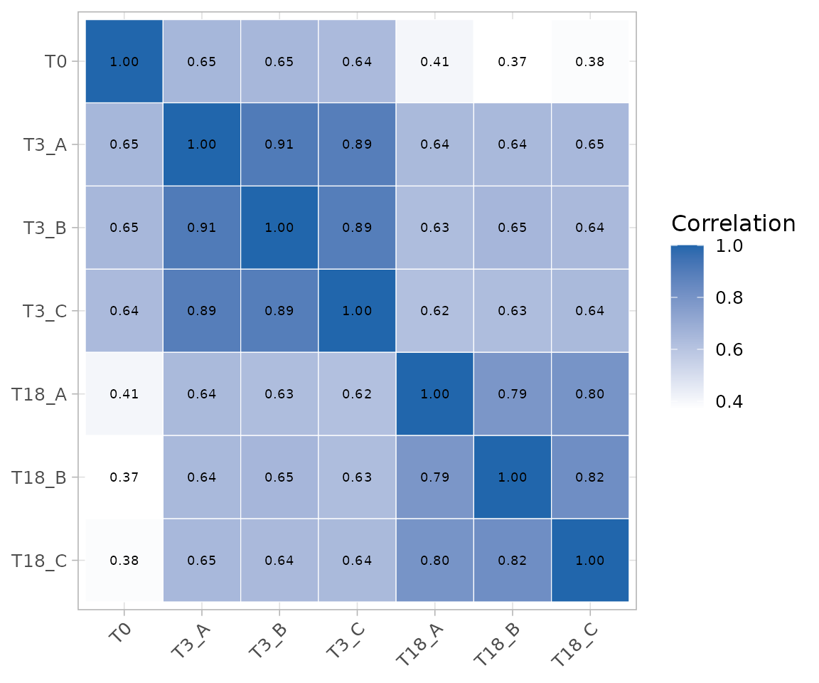

Clustering of the samples

plot_mds() and plot_pca() place the samples so that similar samples are close, and plot_explained_variance() shows how much of the differences between the samples each principal component explains. Both the MDS and the PCA use the log2 normalized counts, with the normalization chosen in normalize_data() (here counts per million), so that the sequencing depth of the samples does not drive the result:

plot_mds(object)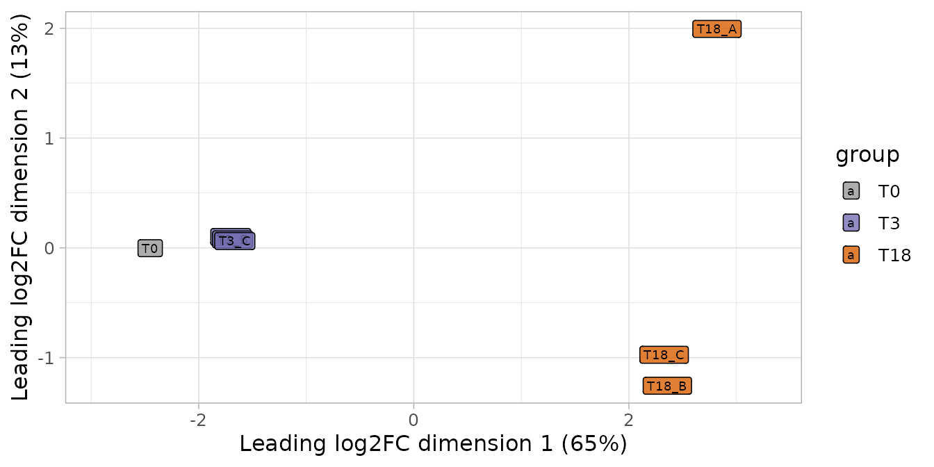

plot_pca(object)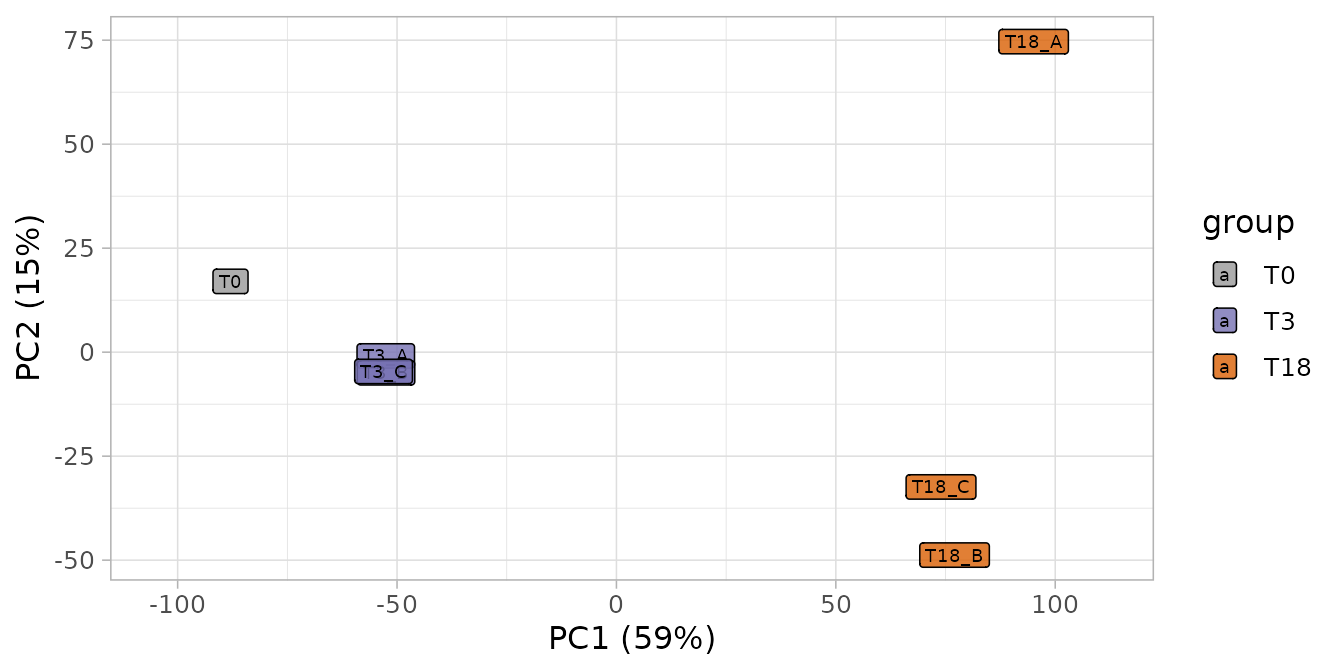

plot_explained_variance(object)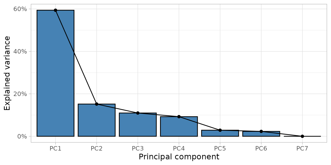

plot_explained_variance(object, cumulative = TRUE)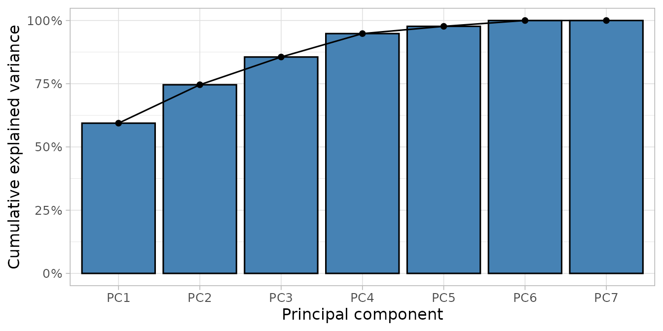

The first dimension of both plots orders the samples by time point (T0, then day 3, then day 18): the main difference between the samples is the growth of the cells, as expected in a dropout screen. The day 3 replicates are very close; the day 18 replicates differ more, because the depletion has had more time to diverge. The first principal component explains 59% of the variability.

Quality with reference genes

The most informative check of a dropout screen uses genes whose behaviour is known: the core essential genes should be depleted, the non-essential genes should not. hart_reference_genes has the lists of Hart et al. for human cells. compute_screen_quality() measures how well the two groups are separated (NNMD and Cohen’s d: more negative is better; ROC AUC: 0.5 is no separation, 1 is perfect) and plot_reference_separation() shows it. The two lists were read above, to classify the lost sgRNAs:

c(`Core essential` = length(essential), `Non-essential` = length(nonessential))
#> Core essential  Non-essential 
#>            684            926

compute_metrics() computes the log2 fold change of each sgRNA between two groups of samples. In a treated screen they are a treatment and a control of the same day; in a dropout screen they are two time points: condition_column = "Day" makes control and treatment values of the Day column.

day3 <- compute_metrics(object,
    control = "T0", treatment = "T3", condition_column = "Day"
)
day18 <- compute_metrics(object,
    control = "T0", treatment = "T18", condition_column = "Day"
)
quality <- bind_rows(
    `Day 3` = compute_screen_quality(day3, essential, nonessential),
    `Day 18` = compute_screen_quality(day18, essential, nonessential),
    .id = "Time point"
)
knitr::kable(quality, digits = 3)

Time point	NEssential	NNonessential	MeanEssential	MeanNonessential	NNMD	CohenD	AUC
Day 3	646	797	-0.722	0.178	-2.510	-1.604	0.881
Day 18	646	797	-2.346	0.358	-7.199	-3.868	0.998

After 3 days the essential genes are only starting to drop out; after 18 days the separation is almost perfect.

plot_reference_separation(day18, essential, nonessential) +
    ggtitle("Day 18 vs T0")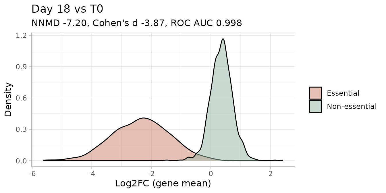

plot_zscore_distribution() compares the sgRNA fold changes of the two time points (the Day column of the tables, T3 and T18). It receives the tables, not the object, so the palette of the time points is given explicitly:

plot_zscore_distribution(list(day3, day18),
    alpha = 0.5, palette = get_palettes(object)$Day
) +
    labs(fill = "Time point")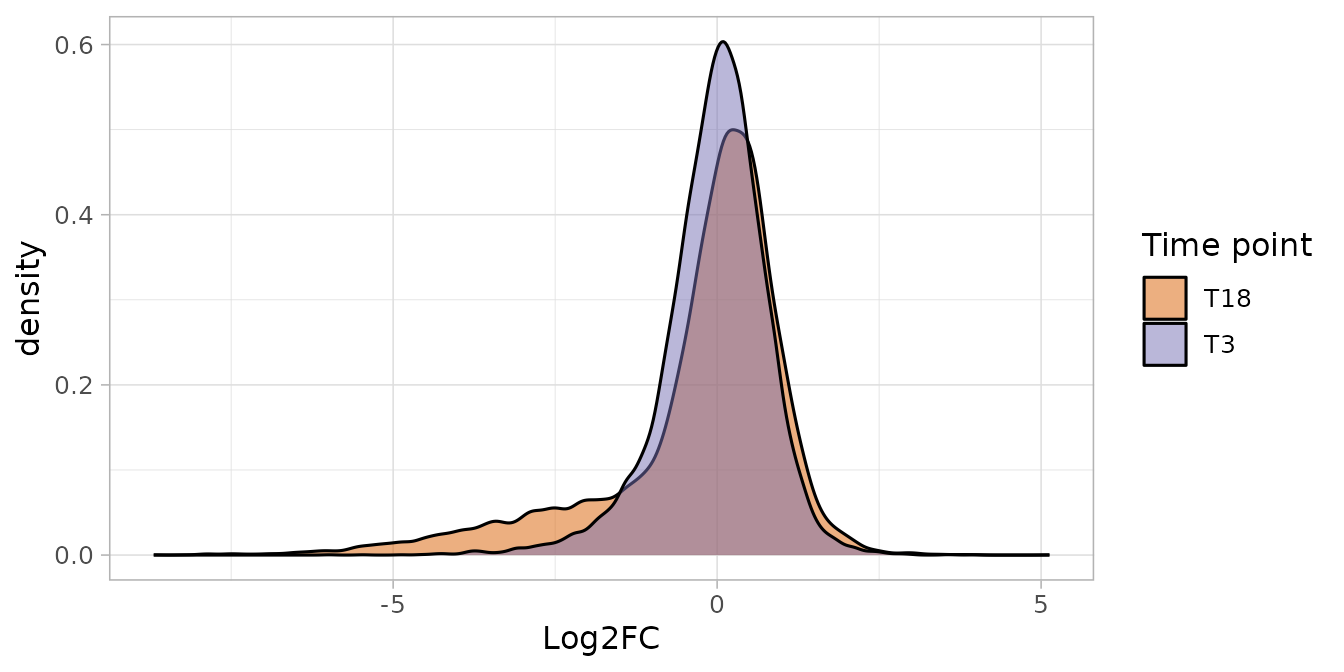

At day 18 the distribution has a long left tail (the depleted sgRNAs) that is only beginning at day 3.

plot_boxplot() shows the normalized counts of the sgRNAs of single genes in each sample, for example two core essential genes and the EGFP control (sgRNAs that target a gene not present in the cells):

plot_boxplot(object,
    genes = c("POLR2L", "RPL14", "EGFP"),
    group_var = "Untreated", fill_var = "Day", ncol = 3
) +
    scale_x_discrete(guide = guide_axis(angle = 45))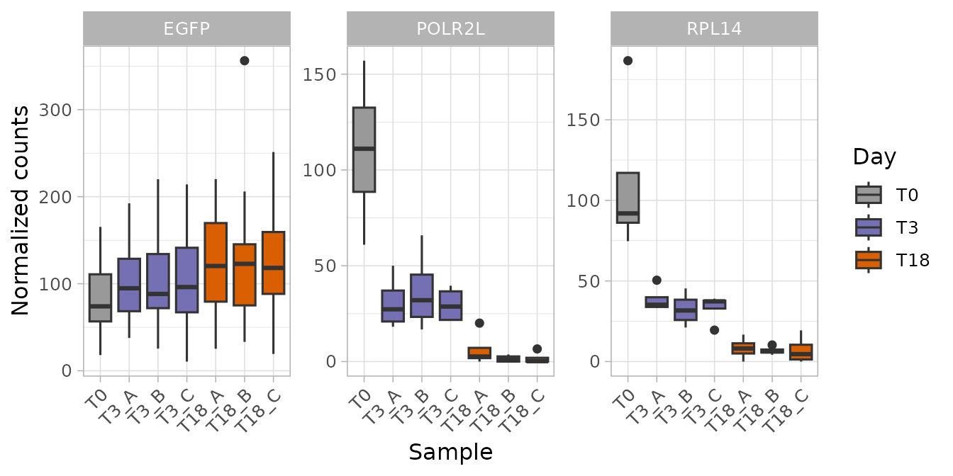

The sgRNAs of the essential genes are depleted at day 3 and almost gone at day 18; those of EGFP are stable (slightly higher, because of the CPM normalization described below).

plot_trend() follows the same genes over time. The time points are in the Day column (time_column, the default), and time places them at their real days, so that day 3 is close to T0 and far from day 18:

plot_trend(object,
    genes = c("POLR2L", "RPL14", "EGFP"), group_var = "Untreated",
    time = c(T0 = 0, T3 = 3, T18 = 18),
    trend = "mean", ncol = 3, scales = "free_y"
) +
    labs(x = "Days", y = "Mean normalized counts per sgRNA")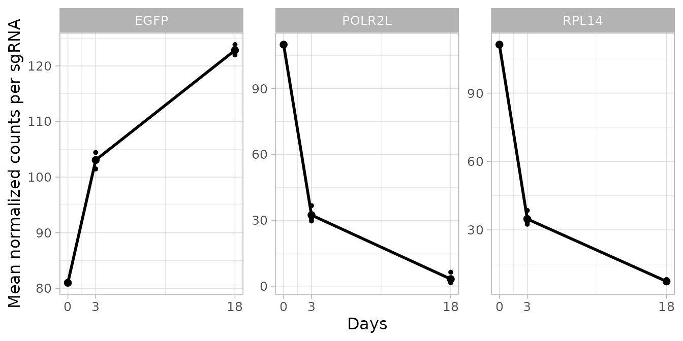

compute_slope() gives the slope of the line of each gene, per day when the real times are given with time: a summary of the depletion rate that can be compared between genes:

compute_slope(object,
    genes = c("POLR2L", "RPL14", "EGFP"), group_var = "Untreated",
    time = c(T0 = 0, T3 = 3, T18 = 18)
)
#> # A tibble: 3 × 2
#> # Rowwise:  Gene
#>   Gene   Slope
#>   <chr>  <dbl>
#> 1 EGFP    1.69
#> 2 POLR2L -3.44
#> 3 RPL14  -3.31

plot_treatment_separation() shows how much a gene changes between two conditions, as the log2 ratio of their mean normalized counts labelled with the percentage difference. Here the conditions are the time points (condition_column = "Day", the same column as time_column), so every time point is compared with T0 and placed at its real day:

plot_treatment_separation(object, genes = c("POLR2L", "RPL14", "EGFP"),
    treatment = c("T3", "T18"), control = "T0", condition_column = "Day",
    time = c(T0 = 0, T3 = 3, T18 = 18), nrow = 1
) +
    labs(x = "Days")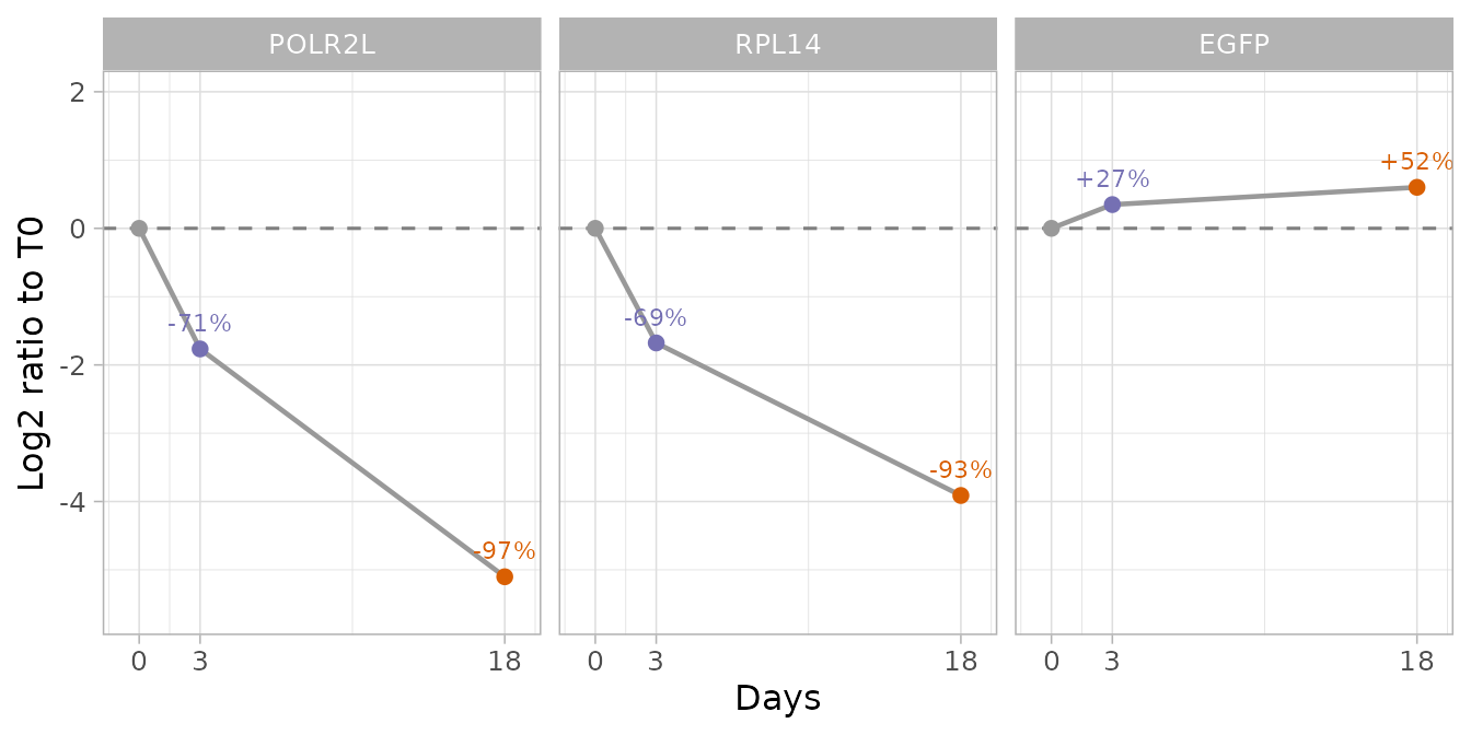

plot_barcode_heatmap() shows each sgRNA in each sample (log2 normalized counts minus the mean of the sgRNA): every sgRNA of the two essential genes drops out, which is what a good knockout looks like. A gene supported by a single sgRNA would show one blue row among white ones.

plot_barcode_heatmap(object, genes = c("POLR2L", "RPL14")) +
    scale_x_discrete(guide = guide_axis(angle = 45))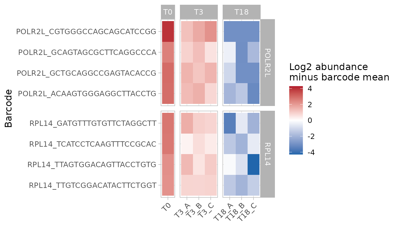

The non-essential genes have a positive mean log2 fold change (0.36 at day 18) although they have no effect. This is a side effect of the CPM normalization: when many sgRNAs drop out, the reads of the sample go to the others, which look enriched. The ranking of the genes does not change, but the baseline is not 0. Normalizing to the sgRNAs of the non-essential genes (method = "control") puts it back at 0:

nonessential_sgrnas <- intersect(rownames(object),
    hap1_annotation_table$Barcode[hap1_annotation_table$Gene %in% nonessential])
day18_control <- normalize_data(object,
    method = "control", control_barcodes = nonessential_sgrnas
) %>%
    compute_metrics(control = "T0", treatment = "T18",
        condition_column = "Day")
knitr::kable(compute_screen_quality(day18_control, essential, nonessential),
    digits = 3)

NEssential	NNonessential	MeanEssential	MeanNonessential	NNMD	CohenD	AUC
646	797	-2.782	0.027	-7.184	-3.688	0.997

The rest of the tutorial uses the CPM normalization. The baseline matters for the self-contained tests such as FRY, which ask whether a gene changes at all: with the non-essential sgRNAs at 0, the small real effects of many genes become significant. In this dataset, normalizing to half of the non-essential genes made FRY call about 6% of the other half at 5% FDR, against almost none with CPM. The tests that compare each gene with the others (CAMERA and the Z-score tests) depend much less on the baseline.

sgRNA efficiency

Not every sgRNA works equally well: some knock out their gene, others have little effect. A dropout screen gives an indirect estimate of this through the core essential genes: all their sgRNAs should be depleted, so an sgRNA of an essential gene that is barely depleted is probably inefficient. It is an estimate, not a measurement: the depletion also depends on how often the repair keeps the gene in frame, on how essential the gene is in these cells and on the noise of the counts. The sequence of each sgRNA (20 nucleotides, before the NGG PAM) is the second part of its identifier, so it can be related to the depletion.

Here an sgRNA of an essential gene is called effective when its log2 fold change at day 18 is below the 5th percentile of the sgRNAs of the non-essential genes. The cut off is a choice: by construction 5% of the sgRNAs without effect would pass it too.

guides <- day18 %>%
    mutate(
        Sequence = sub(".*_", "", Barcode),
        GC = nchar(gsub("[AT]", "", Sequence)) / nchar(Sequence),
        PAMProximal = substr(Sequence, 20, 20)
    )
threshold <- quantile(
    guides$Log2FC[guides$Gene %in% nonessential], 0.05)
essential_guides <- guides %>%
    filter(Gene %in% essential) %>%
    mutate(Effective = Log2FC < threshold)
mean(essential_guides$Effective)
#> [1] 0.8358446

84% of the sgRNAs of the core essential genes are effective. A gene needs only some effective sgRNAs to be found, and most essential genes have three or four:

essential_guides %>%
    group_by(Gene) %>%
    summarise(EffectiveGuides = sum(Effective)) %>%
    dplyr::count(EffectiveGuides)
#> # A tibble: 5 × 2
#>   EffectiveGuides     n
#>             <int> <int>
#> 1               0     6
#> 2               1    24
#> 3               2    87
#> 4               3   206
#> 5               4   323

The genes with no or one effective sgRNA are the ones the gene-level tests are most likely to miss: plot_barcode_heatmap() and plot_barcode_hit() show them as single blue rows among white ones.

Is the difference between the sgRNAs of a gene a property of the sgRNAs, or noise? If it is a property of the sgRNAs it is the same in independent cultures. The three replicates (A, B and C) were grown separately from day 3 to day 18, so the change of each sgRNA in this interval is measured three times independently. The part specific to the sgRNA is its log2 fold change minus the median of its gene:

normalized <- get_normalized_count_table(object)
#> ScreenR normalized count table: 13598 rows, 8 columns
guide_effect <- function(late, early) {
    tibble(
        Gene = hap1_annotation_table$Gene[
            match(normalized$Barcode, hap1_annotation_table$Barcode)],
        Log2FC = log2((normalized[[late]] + 0.5) / (normalized[[early]] + 0.5))
    ) %>%
        group_by(Gene) %>%
        mutate(GuideEffect = Log2FC - median(Log2FC)) %>%
        pull(GuideEffect)
}
reproducibility <- data.frame(
    A = guide_effect("T18_A", "T3_A"),
    B = guide_effect("T18_B", "T3_B"),
    C = guide_effect("T18_C", "T3_C")
)[normalized$Barcode %in% essential_guides$Barcode, ]
round(cor(reproducibility, method = "spearman"), 2)
#>      A    B    C
#> A 1.00 0.37 0.36
#> B 0.37 1.00 0.41
#> C 0.36 0.41 1.00

The correlations are positive in every pair of cultures: part of the difference between the sgRNAs of an essential gene is reproducible, so it belongs to the sgRNAs; the rest is noise. A single screen ranks the sgRNAs only roughly.

The efficiency depends on the sequence. The GC content and the nucleotide next to the PAM (position 20) are two known factors (Doench et al. 2014): sgRNAs with a GC content of about 50-60% and a G at position 20 deplete more.

essential_guides %>%
    mutate(GC = cut(GC, c(0, 0.4, 0.5, 0.6, 0.7, 1),
        labels = c("<40%", "40-50%", "50-60%", "60-70%", ">70%"))) %>%
    ggplot(aes(GC, Log2FC)) +
    geom_boxplot(fill = time_colors[["T18"]], alpha = 0.5,
        outlier.size = 0.5) +
    labs(x = "GC content", y = "Log2FC at day 18",
        title = "sgRNAs of the core essential genes")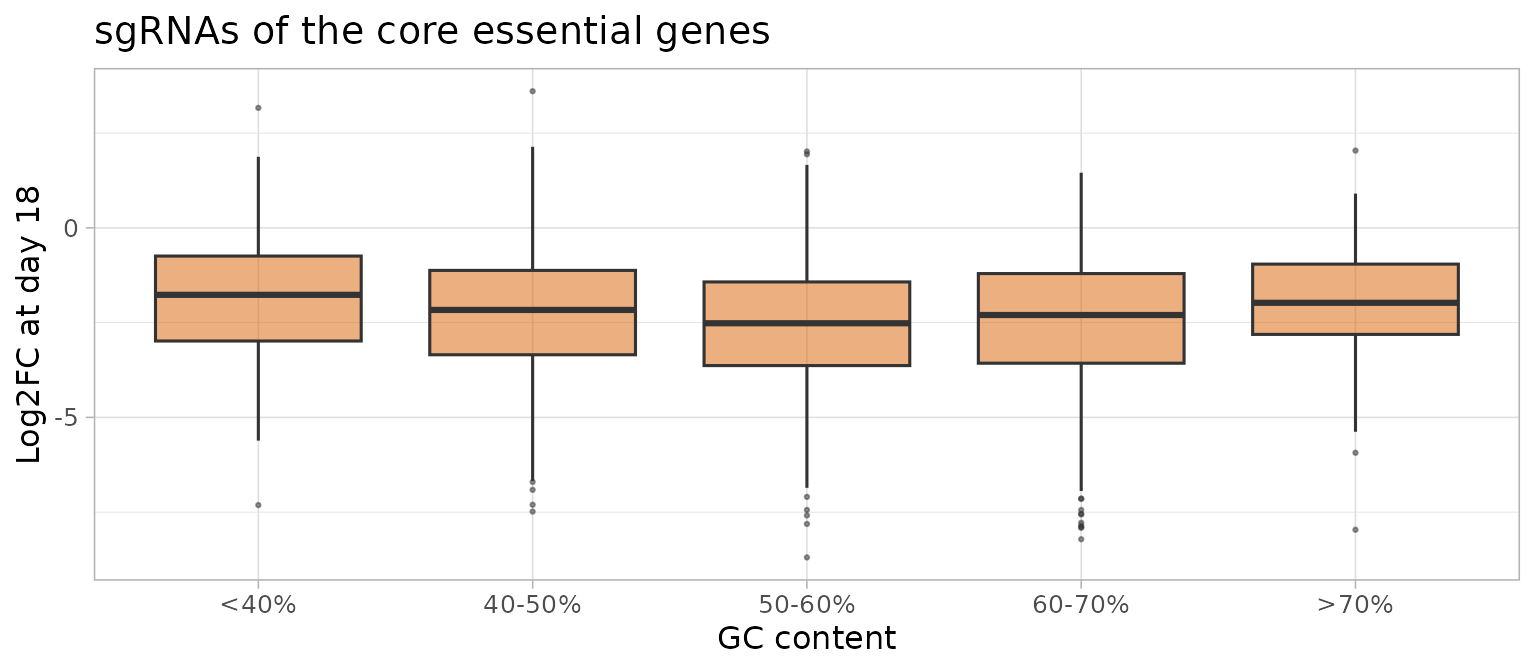

essential_guides %>%
    group_by(PAMProximal) %>%
    summarise(Guides = n(), MedianLog2FC = median(Log2FC),
        Effective = mean(Effective))
#> # A tibble: 4 × 4
#>   PAMProximal Guides MedianLog2FC Effective
#>   <chr>        <int>        <dbl>     <dbl>
#> 1 A              780        -2.09     0.828
#> 2 C              332        -1.80     0.777
#> 3 G             1257        -2.50     0.866
#> 4 T              153        -1.97     0.758

The GC content and the nucleotide at position 20 explain only a small part of the differences: the depletion is a noisy and indirect estimate, and these plots show trends, not the efficiency of a single sgRNA.

None of the sgRNAs contains TTTT (0 sgRNAs), which ends the transcription by the U6 promoter: the library was designed to avoid it. These effects are small compared with the differences between genes, and the gene-level tests do not need them; they are useful to choose the sgRNAs of a validation experiment, or to judge a gene whose sgRNAs disagree (see find_discordant_barcodes() below). For a prediction of the efficiency of an sgRNA use dedicated tools, such as Rule Set 2 (Doench et al. 2016); to measure it, sequence the target site of the cells (the fraction of edited alleles) or check the loss of the protein.

Copy-number bias and CRISPRcleanR

Cas9 cuts the DNA, and cells with many cuts grow less. sgRNAs that target amplified regions of the genome therefore deplete the cells whatever the gene they target, and the genes there look essential. CRISPRcleanR (Iorio et al. 2018) finds the regions where many neighbouring sgRNAs that target different genes are depleted together and corrects their fold changes, without needing copy-number data. correct_crispr_bias() runs CRISPRcleanR on a ScreenR object and returns a new ScreenR object with the corrected counts. ScreenR does not reimplement the method: it only calls CRISPRcleanR.

The correction needs

the complete genome-wide library: CRISPRcleanR assumes that most of the genes in a region have no effect. On a subset of genes enriched in hits it removes real signal, so it must not be used on hap1_count_table;
a library annotation with the position of each sgRNA, in the format of CRISPRcleanR (row names: the sgRNA identifiers; columns GENES, CHRM, STARTpos and ENDpos). CRISPRcleanR includes the annotation of several libraries (KY_Library_v1.0, Brunello_Library, AVANA_Library, GeCKO_Library_v2, …); for another library, build the data frame from its annotation file.

This example uses the complete HT-29 screen distributed with CRISPRcleanR (KY library, about 90,000 sgRNAs; HT-29 cells carry an amplification of the MYC region on chromosome 8q24). It takes about a minute.

ccr <- "CRISPRcleanR"
# Library annotation and counts distributed with CRISPRcleanR
library_annotation <- get(utils::data("KY_Library_v1.0", package = ccr))
counts <- read.delim(system.file("extdata", "HT-29_counts.tsv",
    package = ccr
))
colnames(counts) <- c("Barcode", "Gene", "Plasmid", "HT29_R1", "HT29_R2",
    "HT29_R3")
ht29 <- create_screenr_object(
    table = counts[, -2], annotation = counts[, c("Barcode", "Gene")],
    groups = factor(c("Plasmid", "Late", "Late", "Late")),
    sample_table = data.frame(
        Sample = c("Plasmid", "HT29_R1", "HT29_R2", "HT29_R3"),
        Day = c("Plasmid", "Late", "Late", "Late"), Treatment = "Untreated"
    )
)
ht29_corrected <- correct_crispr_bias(ht29,
    library_annotation = library_annotation,
    control = "Plasmid", treatment = c("HT29_R1", "HT29_R2", "HT29_R3")
)
ht29_corrected

The corrected object is analysed like any other: normalize it, compute the data table and find the hits. CRISPRcleanR’s own results (the corrected sgRNA fold changes and the segments of the genome) are in S4Vectors::metadata(ht29_corrected)$crisprcleanr.

The effect of the correction on this screen (computed with the code above; the script is in the benchmark/crispr folder of the GitHub repository):

correction <- read.csv(system.file("extdata", "crisprcleanr_ht29.csv",
    package = "ScreenR"
))
knitr::kable(correction, digits = 3,
    col.names = c("Counts", "NNMD", "Cohen's d", "ROC AUC",
        "Mean log2FC in 8q24 (genes not known to be essential)")
)

Counts	NNMD	Cohen’s d	ROC AUC	Mean log2FC in 8q24 (genes not known to be essential)
Raw	-8.288	-2.947	0.994	-0.260
Corrected (CRISPRcleanR)	-8.765	-2.617	0.979	0.019

Before the correction, the genes in the amplified 8q24 region that are not known to be essential are depleted (mean log2 fold change about -0.26); after the correction they are not (about 0). The separation of the reference genes is similar, with a slightly lower ROC AUC: the correction removes a gene-independent bias, it does not make the screen stronger.

Finding the hits

The hit-finding functions are used as in Tutorial 3. The comparison is day 18 against T0:

design <- create_design_matrix(object)
contrast <- create_contrast(design, treatment = "T18", control = "T0")

Gene-level Z-score test with the non-essential genes as reference

find_gene_zscore_hit() compares the mean score of the sgRNAs of each gene with the scores of random sets of sgRNAs. By default the random sgRNAs come from all the genes, which include the hits, so the test is conservative when many genes have an effect, as in proliferation screens. When genes known to have no effect are available, they are a better reference (control_genes). For CRISPR screens the non-essential genes are the natural choice: their sgRNAs cut the DNA like any other, while non-targeting sgRNAs do not.

To be able to check the result, here half of the non-essential genes are used as reference and the other half is kept to count the false calls; in a real analysis use all of them.

set.seed(2017)
reference <- sample(nonessential, length(nonessential) %/% 2)
held_out <- setdiff(nonessential, reference)
statistics <- compute_barcode_statistics(object, design, contrast)
zscore <- find_gene_zscore_hit(statistics,
    control_genes = reference, fdr = 1, seed = 1
)
head(zscore)
#> # A tibble: 6 × 6
#>   Gene   NBarcodes Score Log2FC     PValue       FDR
#>   <chr>      <int> <dbl>  <dbl>      <dbl>     <dbl>
#> 1 AARS           4 -2.73  -2.41 0.00001000 0.0000476
#> 2 ABCE1          4 -3.17  -3.15 0.00001000 0.0000476
#> 3 ABCF1          4 -2.37  -1.74 0.00001000 0.0000476
#> 4 ACTR10         4 -3.47  -3.18 0.00001000 0.0000476
#> 5 ACTR2          4 -2.94  -2.21 0.00001000 0.0000476
#> 6 ADSL           4 -3.52  -3.07 0.00001000 0.0000476

called <- zscore$Gene[zscore$FDR <= 0.05]
data.frame(
    `Genes called` = length(called),
    `Core essential` = sum(called %in% essential),
    `Held-out non-essential` = sum(called %in% held_out),
    `Other genes` = sum(!called %in% c(essential, nonessential)),
    check.names = FALSE
)
#>   Genes called Core essential Held-out non-essential Other genes
#> 1          911            619                      5         287

Almost all the 646 core essential genes of the dataset are found at 5% FDR, with very few of the held-out non-essential genes. The other genes called are not in the reference lists: HAP1 cells need many more genes than the core essential set, which contains only the genes essential in almost every cell line.

Without reference genes: the empirical null

When no reference genes are available, reference = "empirical" estimates the scores of the genes without effect from the data. Most genes have no effect, so the centre of the distribution of the gene statistics is the null; a normal distribution is fitted there and gives the p-values. The hits, in the tail, do not widen it. empirical_fit = "one-sided" estimates the spread from the side without hits only (above the centre for depleted genes), which gives more power when the hits are well separated, as in CRISPR screens; the default, "central", is the safer choice (see ?find_gene_zscore_hit).

zscore_empirical <- find_gene_zscore_hit(statistics,
    reference = "empirical", fdr = 1
)
zscore_one_sided <- find_gene_zscore_hit(statistics,
    reference = "empirical", empirical_fit = "one-sided", fdr = 1
)
attr(zscore_one_sided, "null")
#>      mean        sd 
#> 0.5670556 0.6900248

plot_empirical_null() shows the gene statistics and the fitted null, which should follow the centre of the distribution; the depleted genes are in the tail on the left:

plot_empirical_null(statistics, empirical_fit = "one-sided")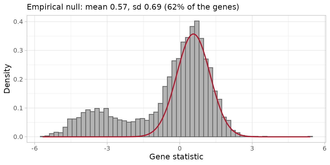

Other methods and their consensus

The other methods need no reference genes either: the default reference of the Z-score test (random sets of sgRNAs of all the genes), CAMERA and FRY. number_barcode = 2 keeps the genes with 3 or 4 sgRNAs.

zscore_default <- find_gene_zscore_hit(statistics, fdr = 1, seed = 1)
camera <- find_camera_hit(object, design, contrast,
    number_barcode = 2, fdr = 1
)
fry <- find_roast_hit(object, design, contrast,
    method = "fry", number_barcode = 2, fdr = 1
)
hit_list <- list(zscore_reference = zscore,
    zscore_empirical = zscore_empirical,
    zscore_one_sided = zscore_one_sided, zscore = zscore_default,
    camera = camera, fry = fry)
hits <- summarise_hits(hit_list, fdr = 0.05)
head(hits)
#> # A tibble: 6 × 10
#>   Gene    FDR_zscore_reference FDR_zscore_empirical FDR_zscore_one_sided
#>   <chr>                  <dbl>                <dbl>                <dbl>
#> 1 ATP6V1F            0.0000476         0.0000000236             4.47e-14
#> 2 BUB3               0.0000476         0.0000000130             1.47e-14
#> 3 CPSF1              0.0000476         0.0000000345             9.08e-14
#> 4 DHX15              0.0000476         0.0000000102             8.10e-15
#> 5 DPAGT1             0.0000476         0.0000000262             5.44e-14
#> 6 EIF3A              0.0000476         0.0000000101             6.35e-15
#> # ℹ 6 more variables: FDR_zscore <dbl>, FDR_camera <dbl>, FDR_fry <dbl>,
#> #   NMethods <dbl>, MaxFDR <dbl>, Hit <lgl>
table(hits$NMethods)
#> 
#>    0    1    2    3    4    5    6 
#> 2415   22   98  121  294   69  332

plot_volcano() shows all the genes: the hits found by every method are above the dashed line, on the left (depleted). The core essential gene POLR2L is circled:

plot_volcano(hits, statistics = statistics, fdr = 0.05, genes = "POLR2L")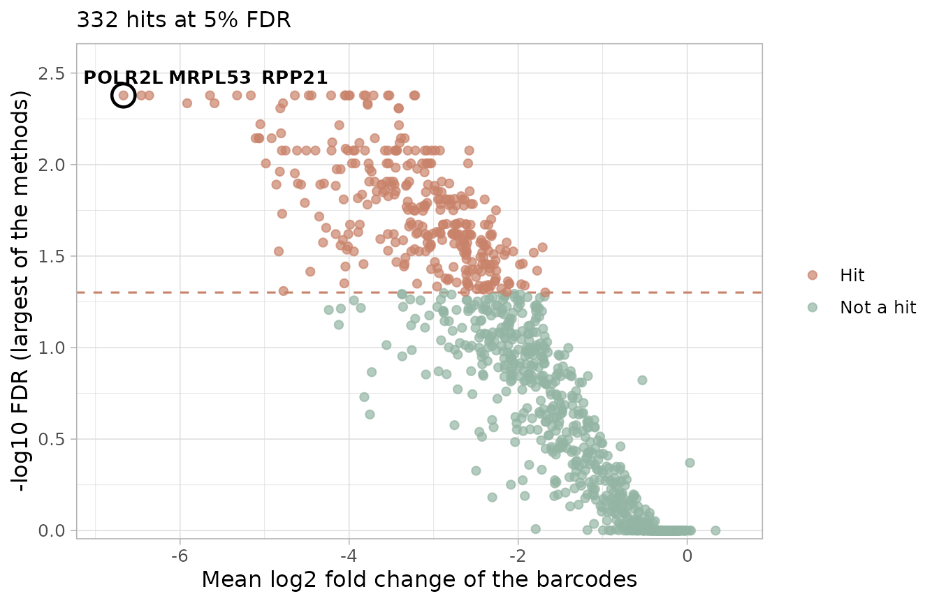

plot_common_hit() shows how the hits of the methods overlap (an UpSet plot, since there are more than three methods; each column counts the genes found by exactly the combination of methods marked below it):

plot_common_hit(hit_list, fdr = 0.05,
    title = "Depleted genes at day 18 (5% FDR)")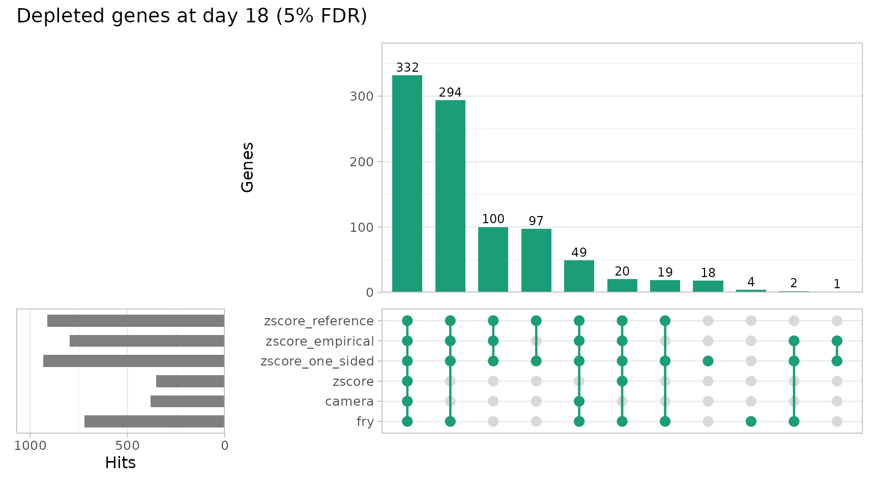

find_common_hit() returns the genes found by at least common_in methods, for example by all six:

common <- find_common_hit(hit_list, fdr = 0.05)
length(common)
#> [1] 332
mean(common %in% essential)
#> [1] 0.8674699

How many of the hits are core essential, and how many are held-out non-essential genes (false calls):

evaluate_hits <- function(result) {
    called <- result$Gene[result$FDR <= 0.05]
    data.frame(
        `Genes called` = length(called),
        `Core essential` = sum(called %in% essential),
        `Held-out non-essential` = sum(called %in% held_out),
        check.names = FALSE
    )
}
knitr::kable(bind_rows(lapply(hit_list, evaluate_hits), .id = "Method"))

Method	Genes called	Core essential	Held-out non-essential
zscore_reference	911	619	5
zscore_empirical	798	596	3
zscore_one_sided	932	619	7
zscore	352	305	0
camera	381	326	0
fry	720	552	1

The empirical null finds almost as many core essential genes as the non-essential reference, without reference genes and with very few held-out non-essential genes. The two tests that compare each gene with all the others (the default Z-score test and CAMERA) are much more conservative: they find less than half of the core essential genes, and the default Z-score test does not give a p-value below 0.05 to any of the held-out non-essential genes. Their reference is all the genes of the library, and here it is full of hits: the subset keeps all the reference genes, so 19% of its genes are core essential, against about 4% in the complete TKOv3 library. They remain conservative on the complete library: there the default Z-score test found 58% of the core essential genes at 5% FDR, the empirical null 90% ("central") and 94% ("one-sided"), and the non-essential reference 96%. The default Z-score test and CAMERA rank the genes almost in the same way (Spearman correlation of the p-values above 0.99).

FRY (find_roast_hit()) tests each gene on its own sgRNAs. It estimates the variability from the replicates of the model, so a single T0 sample is enough when the other time points have replicates, as here. It finds more essential genes than the tests without reference, with very few held-out non-essential genes.

Depleted at every time point

find_consistent_hit() runs the same method for several contrasts and calls a gene only if it is depleted in all of them (the p-value of the gene is the largest of its p-values). Here the contrasts are day 3 and day 18 against T0, with FRY:

contrast_day3 <- create_contrast(design, treatment = "T3", control = "T0")
consistent <- find_consistent_hit(object, design,
    contrasts = list(Day3 = contrast_day3, Day18 = contrast),
    method = "fry", method_args = list(number_barcode = 2), fdr = 1
)
head(consistent)
#> # A tibble: 6 × 9
#>   Gene  Direction NContrasts  PValue    FDR PValue_Day3 Log2FC_Day3 PValue_Day18
#>   <chr> <chr>          <int>   <dbl>  <dbl>       <dbl>       <dbl>        <dbl>
#> 1 RPA2  Down               2 9.13e-6 0.0306  0.00000913      -2.34   0.00000203 
#> 2 RTF1  Down               2 2.14e-5 0.0346  0.0000214       -0.568  0.000000779
#> 3 RPL23 Down               2 4.00e-5 0.0346  0.0000400       -1.51   0.0000337  
#> 4 RPL14 Down               2 5.71e-5 0.0346  0.0000571       -1.47   0.00000141 
#> 5 SMU1  Down               2 6.02e-5 0.0346  0.0000260       -3.34   0.0000602  
#> 6 CKAP5 Down               2 6.19e-5 0.0346  0.0000574       -1.75   0.0000619  
#> # ℹ 1 more variable: Log2FC_Day18 <dbl>

Only 15 genes pass 5% FDR, because at day 3 the depletion is only beginning and FRY, which uses the variability of the replicates, has little power there. The genes found (13 of them are core essential) are those whose loss stops the growth of the cells immediately, such as the ribosomal proteins. combine_consistent_hits() does the same with tables of p-values computed beforehand, for example with different methods for each contrast.

A dropout screen has no treatment, so the methods that compare treated and control samples over time, find_time_hit() and filter_by_slope(), are not used here; they are useful in screens with a drug and a vehicle arm at several time points (see Tutorial 3).

Looking at single genes

Before validating a hit, look at its sgRNAs: a convincing knockout has all its sgRNAs depleted, not only one. Take the ten best genes found by all the methods that are not in the reference lists:

candidates <- hits %>%
    filter(NMethods == length(hit_list),
        !Gene %in% c(essential, nonessential)) %>%
    arrange(MaxFDR) %>%
    head(10) %>%
    pull(Gene)
candidates
#>  [1] "ATP6V1F" "PPP6C"   "DUT"     "EIF1AD"  "SLC30A9" "UBE2S"   "NDNL2"  
#>  [8] "NAA25"   "MRPL13"  "COX7C"

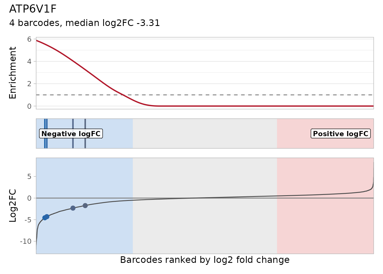
plot_barcode_hit() ranks all the sgRNAs by their log2 fold change (day 18 against T0, from the model) and marks the sgRNAs of the gene (vertical lines): lines on the left side mean that the gene is depleted. As in the hit-finding functions, number_barcode = 2 accepts genes with 3 sgRNAs:

plot_barcode_hit(object, design, contrast,
    number_barcode = 2, gene = candidates[1]
)

plot_barcode_trend() follows the log2 fold change of each sgRNA at day 3 and day 18 (from the tables of compute_metrics(), in the order of the list). With n_col larger than 1 it combines the plots of the genes (a patchwork object, so & applies a theme to all of them), here the first three; each line is an sgRNA, and the long sgRNA names of the legend are hidden:

plot_barcode_trend(list(day3, day18), genes = candidates[1:3], n_col = 3) &
    theme(legend.position = "none")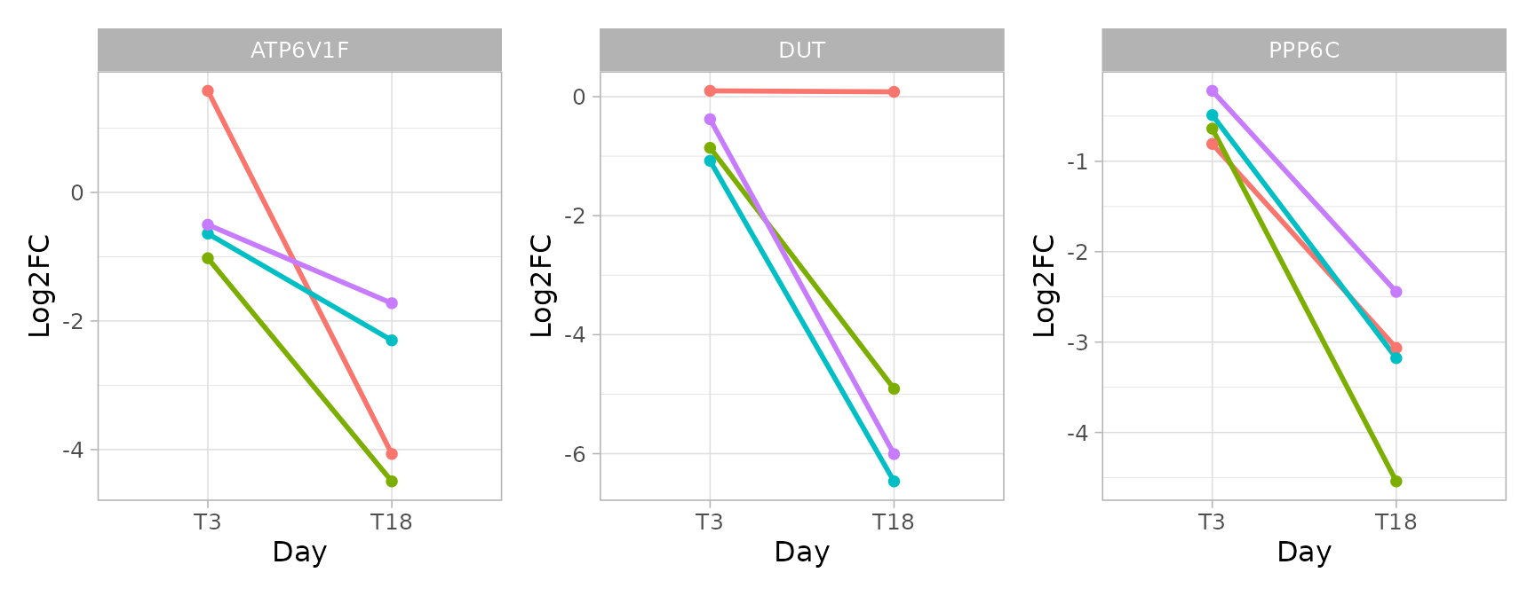

plot_barcode_heatmap() shows the sgRNAs of all ten genes in every sample, next to a core essential gene for comparison:

plot_barcode_heatmap(object, genes = c(candidates, "POLR2L")) +
    scale_x_discrete(guide = guide_axis(angle = 45))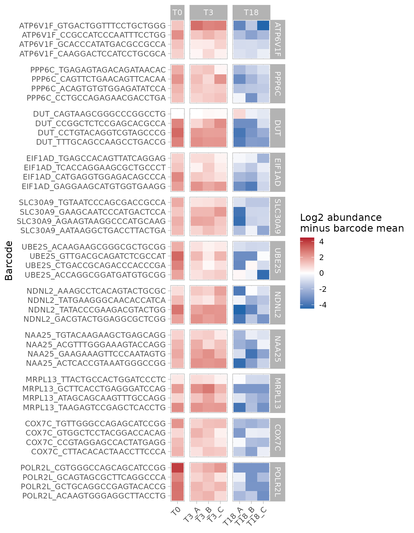

find_discordant_barcodes() lists the sgRNAs that behave very differently from the other sgRNAs of their gene (distance from the median of the gene in units of its MAD). With 3 or 4 sgRNAs per gene the MAD is unstable, so many sgRNAs pass the default threshold: use it to look at the hits, not to filter the library, and do not remove sgRNAs before the tests.

discordant <- find_discordant_barcodes(day18, threshold = 3)
filter(discordant, Gene %in% common)
#> # A tibble: 73 × 5
#>    Barcode                     Gene    Log2FC GeneLog2FC Deviation
#>    <fct>                       <chr>    <dbl>      <dbl>     <dbl>
#>  1 MRPL53_GGCGGTGAGCATTTCCAGAG MRPL53 -7.10        -4.02     -27.4
#>  2 CCT8_TTTGCCCAGATGCTCAAGGA   CCT8   -4.19        -1.70     -24.4
#>  3 MRPL39_GAGGAGGTACGACTCAGGCG MRPL39  0.0621      -3.39      21.4
#>  4 DKC1_ACAAGGATGAGAGTTACCTG   DKC1   -4.67        -2.93     -20.1
#>  5 PPP1R8_TTGGGCAGTCGAACAGCGGG PPP1R8 -0.774       -3.28      19.0
#>  6 SYMPK_CATGACCCAGCTCTACAAGG  SYMPK  -5.07        -2.41     -17.8
#>  7 GEMIN5_AAACAATCTTCACCAGGCAG GEMIN5 -0.988       -3.90      16.8
#>  8 RPP21_CTGGAGCGCGGCGGTGATGG  RPP21  -2.74        -4.86      13.3
#>  9 CDK9_GCACCGCAAGACCGGCCAGA   CDK9   -8.22        -2.07     -12.9
#> 10 ELP2_CAAGATAGTGATCTTCCAGA   ELP2   -3.01        -1.94     -11.5
#> # ℹ 63 more rows

filter_by_variance() keeps the genes whose sgRNAs agree (variance of the sgRNA log2 fold changes, from the model, below variance):

filter_by_variance(object,
    genes = candidates, matrix_model = design, contrast = contrast,
    variance = 0.5
) %>%
    distinct(Gene, Variance)
#> # A tibble: 10 × 2
#>    Gene    Variance
#>    <chr>      <dbl>
#>  1 EIF1AD    2.28  
#>  2 NAA25     1.10  
#>  3 NDNL2     3.57  
#>  4 DUT      10.3   
#>  5 UBE2S     1.14  
#>  6 SLC30A9   0.0734
#>  7 COX7C     1.02  
#>  8 ATP6V1F   1.99  
#>  9 MRPL13   12.9   
#> 10 PPP6C     1.05

Comparable fold changes

scale_by_reference() scales the fold changes so that the non-essential genes are at 0 and the essential genes at -1. Scaled values can be compared between screens of different strength, for example between cell lines or time points:

scaled <- scale_by_reference(day18, essential, nonessential)
scaled %>%
    group_by(Gene) %>%
    summarise(ScaledLog2FC = mean(ScaledLog2FC)) %>%
    arrange(ScaledLog2FC) %>%
    head()
#> # A tibble: 6 × 2
#>   Gene    ScaledLog2FC
#>   <chr>          <dbl>
#> 1 POLR2L         -2.23
#> 2 POLR3H         -2.15
#> 3 GPN3           -2.11
#> 4 ISG20L2        -1.94
#> 5 RRM1           -1.93
#> 6 MRPL53         -1.91

Positive-selection screens

In a drug-resistance or positive-selection screen the interesting genes are enriched: their knockout makes the cells survive. Every hit-finding function takes direction = "Up":

find_gene_zscore_hit(statistics, direction = "Up")
find_camera_hit(object, design, contrast, direction = "Up")

The reference genes are not useful there (they describe fitness, not resistance); use the default reference of find_gene_zscore_hit() or control genes known to have no effect on the selection.

Summary

Step	CRISPR-specific advice	Functions
Create the object	time points in the Day column of a `sample_table`, one Treatment for all the samples	`create_screenr_object()`
sgRNAs per gene	lower `number_barcode` / `min_barcodes` for 3-6 sgRNAs per gene	`barcodes_per_gene()`
Compare time points	`condition_column = "Day"`	`compute_metrics()`, `plot_treatment_separation()`
Quality control	lost sgRNAs at the late time point are expected; check the separation of essential and non-essential genes	`barcode_lost()`, `plot_barcode_lost()`, `plot_barcode_lost_for_gene()`, `compute_screen_quality()`, `plot_reference_separation()`, `plot_zscore_distribution()`, `plot_trend()`, `compute_slope()`, `plot_treatment_separation()`, `plot_barcode_heatmap()`
sgRNA efficiency	the sgRNAs of the essential genes estimate it; check that it is reproducible and relate it to the sequence	`compute_metrics()`, `get_normalized_count_table()`
Copy-number bias	correct with CRISPRcleanR on the complete library	`correct_crispr_bias()`
Hits	use the non-essential genes as reference when available, otherwise the empirical null	`find_gene_zscore_hit(control_genes = )`, `find_gene_zscore_hit(reference = "empirical")`, `plot_empirical_null()`, `find_camera_hit()`, `find_roast_hit()`, `summarise_hits()`, `plot_volcano()`, `plot_common_hit()`, `find_common_hit()`, `find_consistent_hit()`
Single genes	check that all the sgRNAs of a hit agree	`plot_barcode_hit()`, `plot_barcode_trend()`, `plot_barcode_heatmap()`, `find_discordant_barcodes()`, `filter_by_variance()`
Compare screens	scale to the reference genes	`scale_by_reference()`
Positive selection	look for enriched genes	`direction = "Up"`

Literature

Doench JG, Hartenian E, Graham DB et al. (2014). Rational design of highly active sgRNAs for CRISPR-Cas9-mediated gene inactivation. Nat Biotechnol 32:1262-1267.
Doench JG, Fusi N, Sullender M et al. (2016). Optimized sgRNA design to maximize activity and minimize off-target effects of CRISPR-Cas9. Nat Biotechnol 34:184-191.
Hart T, Tong AHY, Chan K et al. (2017). Evaluation and design of genome-wide CRISPR/SpCas9 knockout screens. G3 7:2719-2727.
Hart T, Brown KR, Sircoulomb F, Rottapel R, Moffat J (2014). Measuring error rates in genomic perturbation screens: gold standards for human functional genomics. Mol Syst Biol 10:733.
Iorio F, Behan FM, Goncalves E et al. (2018). Unsupervised correction of gene-independent cell responses to CRISPR-Cas9 targeting. BMC Genomics 19:604.

Session info

sessionInfo()
#> R version 4.6.1 (2026-06-24)
#> Platform: x86_64-pc-linux-gnu
#> Running under: Ubuntu 26.04.1 LTS
#> 
#> Matrix products: default
#> BLAS:   /usr/lib/x86_64-linux-gnu/openblas-pthread/libblas.so.3 
#> LAPACK: /usr/lib/x86_64-linux-gnu/openblas-pthread/libopenblasp-r0.3.32.so;  LAPACK version 3.12.0
#> 
#> locale:
#>  [1] LC_CTYPE=C.UTF-8       LC_NUMERIC=C           LC_TIME=C.UTF-8       
#>  [4] LC_COLLATE=C.UTF-8     LC_MONETARY=C.UTF-8    LC_MESSAGES=C.UTF-8   
#>  [7] LC_PAPER=C.UTF-8       LC_NAME=C              LC_ADDRESS=C          
#> [10] LC_TELEPHONE=C         LC_MEASUREMENT=C.UTF-8 LC_IDENTIFICATION=C   
#> 
#> time zone: UTC
#> tzcode source: system (glibc)
#> 
#> attached base packages:
#> [1] stats     graphics  grDevices utils     datasets  methods   base     
#> 
#> other attached packages:
#> [1] ggplot2_4.0.3    dplyr_1.2.1      ScreenR_1.15.16  BiocStyle_2.40.0
#> 
#> loaded via a namespace (and not attached):
#>  [1] SummarizedExperiment_1.42.0 gtable_0.3.6               
#>  [3] xfun_0.62                   bslib_0.12.0               
#>  [5] htmlwidgets_1.6.4           Biobase_2.72.0             
#>  [7] lattice_0.22-9              vctrs_0.7.3                
#>  [9] tools_4.6.1                 generics_0.1.4             
#> [11] stats4_4.6.1                tibble_3.3.1               
#> [13] pkgconfig_2.0.3             Matrix_1.7-5               
#> [15] RColorBrewer_1.1-3          S7_0.2.2                   
#> [17] desc_1.4.3                  S4Vectors_0.50.3           
#> [19] lifecycle_1.0.5             compiler_4.6.1             
#> [21] farver_2.1.2                stringr_1.6.0              
#> [23] textshaping_1.0.5           statmod_1.5.2              
#> [25] Seqinfo_1.2.0               htmltools_0.5.9            
#> [27] sass_0.4.10                 yaml_2.3.12                
#> [29] tidyr_1.3.2                 pillar_1.11.1              
#> [31] pkgdown_2.2.1               jquerylib_0.1.4            
#> [33] DelayedArray_0.38.2         cachem_1.1.0               
#> [35] limma_3.68.5                abind_1.4-8                
#> [37] tidyselect_1.2.1            locfit_1.5-9.12            
#> [39] digest_0.6.39               stringi_1.8.9              
#> [41] purrr_1.2.2                 bookdown_0.48              
#> [43] labeling_0.4.3              fastmap_1.2.0              
#> [45] grid_4.6.1                  cli_3.6.6                  
#> [47] SparseArray_1.12.3          magrittr_2.0.5             
#> [49] patchwork_1.3.2             S4Arrays_1.12.1            
#> [51] utf8_1.2.6                  withr_3.0.3                
#> [53] edgeR_4.10.7                scales_1.4.0               
#> [55] rmarkdown_2.32              XVector_0.52.0             
#> [57] matrixStats_1.5.0           otel_0.2.0                 
#> [59] ragg_1.5.2                  evaluate_1.0.5             
#> [61] knitr_1.52                  GenomicRanges_1.64.0       
#> [63] IRanges_2.46.0              rlang_1.3.0                
#> [65] glue_1.8.1                  BiocManager_1.30.27        
#> [67] BiocGenerics_0.58.1         jsonlite_2.0.0             
#> [69] R6_2.6.1                    MatrixGenerics_1.24.0      
#> [71] systemfonts_1.3.2           fs_2.1.0

Emanuel Michele Soda

Elena Ceccacci

2026-10-25